Modeling weak snow layer fracture in propagation saw test using an ice column model

Figures & data

Figure 1. (a) Geometrical model of 2.5-cm-thick surface hoar layer (based on surface hoar layer image presented by Jamieson and Schweizer 2000) and (b) stress–displacement curve for ice properties considered for the weak layer model.

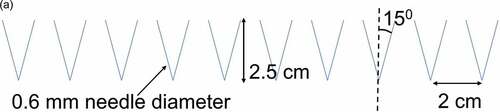
Figure 1. (Continued).

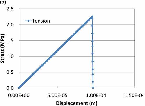
Table 1. Mechanical properties of ice used in the weak layer model.

Ice density = 917 kg/m^3, Elastic modulus = 950 MPa

Yield stress (σy) = 2.25 MPa, plasticity hardening modulus = 95 MPa

Plastic strain at which damage initiates (ε0^pl) =3 × 10^−6, fracture energy of ice (Gf) = 1.05 J/m^2

Figure 2. Finite element model with boundary conditions for estimating the effective mechanical behavior of the surface hoar layer when replaced by a continuum weak layer. DOF = degrees of freedom.

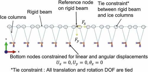
Figure 3. (a) Boundary conditions for numerical propagation saw test (PST) and (b) identification of crack tip.

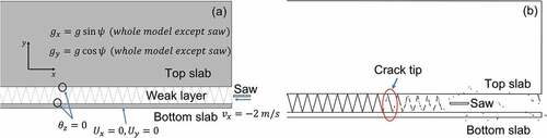
Table 2. Details of parameters used for numerical propagation saw test (PST) simulations.

1. PST model dimensions
Snow layers: Length, 3.5 m; width, 0.005 m. Cutting saw: Length, 0.04 m; width, 0.005 m
2. Snow layers and cutting saw properties
Snow layer	Thickness (m)	Element type	Mechanical model	Density (kg/m^3)	E (MPa)	v
Top slab	0.2–1.0	Plane stress	Elastic	100–500	0.1–50	0.2
Bottom slab	0.01–1.0	Plane stress	Elastic	300	4	0.2
Weak layer	0.005–0.04	Two-dimensional beam	Elastoplastic damage	Given in Table 1
Cutting saw	0.004	Plane stress	Elastic	7,800	1.0E+05	0.3

Figure 4. Effective mechanical behavior of the weak layer. (a) Variation in ice column radius with the weak layer thickness, (b) stress–strain curves for the 4-cm-thick weak layer, (c) variation in the elastic and shear moduli with weak layer thickness, (d) failure curves of weak layers of different thicknesses (negative normal stress represent compression), (e) variation in the weak layer fracture energy with weak layer thickness (tension, compression, and shear modes), and (f) variation in the weak layer fracture energy with loading angle with respect to slope normal (for the 4-cm-thick weak layer).

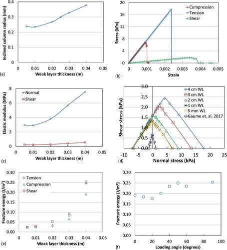
Figure 5. Variation in CCL with (a) top slab density ρ, (b) top slab thickness D, (c) top slab elastic modulus E, (d) bottom slab thickness D_b, (e) weak layer thickness D_wl, (f) slope angle ψ. W_f = weak layer fracture energy; AM = analytical model; DEM = discrete element model; FEM = finite element model; CCL = critical crack length.

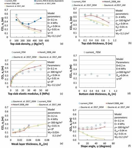
Figure 6. Variation in FPS with fracture propagation distance. (a) Effect of top snow slab density (kg/m³) and (b) effect of friction between top and bottom slabs. FPS = fracture propagation speed; mu: friction coefficient.

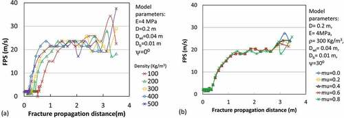
Figure 7. Variation in average FPS with (a) top slab density (experimental data) ρ, (b) top slab density (model results) ρ, (c) top slab thickness D, (d) top slab elastic modulus E, (e) weak layer thickness D_wl, (f) slope angle ψ. ce = elastic wave speed, $(\approx \sqrt{E/\rho }$), shown with dashed line in each figure. DEM = discrete element model; FEM = finite element model; PST = propagation saw test; SWM = solitary wave model; ECT = extended column test; FPS = fracture propagation speed; Exp = experimental.

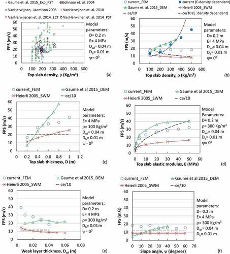
Figure 8. (a) Variation in gravitational work W (top slab), strain energy U_e (whole model), released potential energy (U_e − W) (whole model), kinetic energy K (top slab), and dissipation energy DMD + PD (weak layer) with fracture propagation distance along with CCL (0.2756 m). (b) Variation in specific energies (gravitational work, dW/da [top slab]; PERR, d(U_e − W)/da [shown positive for comparison]; strain energy, dU_e/da [whole model]; kinetic energy, dK/da (top slab), dissipation energy, d(DMD + PD)/da [weak layer]) and maximum crack tip stress with the fracture propagation distance along with CCL. CCL = critical crack length; TS: top slab; WM: whole model; WL: weak layer; PERR: potential energy release rate; DMD: damage dissipation energy; PD: plastic dissipation energy.

Figure 9. (a) Variation in kinetic energy (top slab), dissipation energy (weak layer), and FPS with fracture propagation distance, (b) influence of the top slab elastic modulus on FPS, (c) influence of the top slab elastic modulus on the kinetic energy of the top slab, and (d) influence of the top slab density on the kinetic energy of the top slab. TS = top slab; WL = weak layer; FPS = fracture propagation speed.

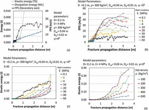
Figure A1. Variation in potential energy release rate with slope angle. D = top slab thickness; E = top slab elastic modulus; ρ = top slab density; D_wl = weak layer thickness; D_b = bottom slab thickness; a = crack size.

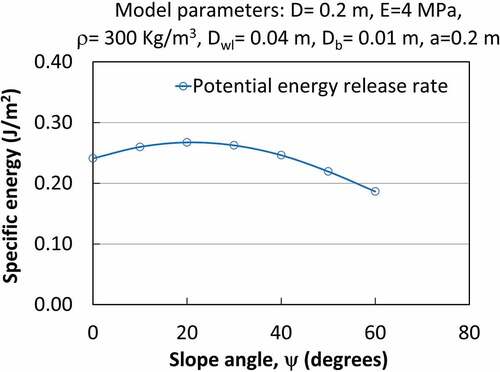
Figure A2. Effect of saw speed on PST simulation results. CCL: Critical crack length; FPS: Fracture propagation speed; PST: Propagation saw test.

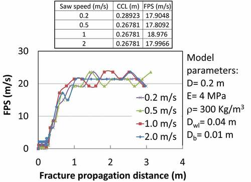
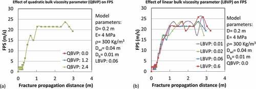
Figure A3. Effect of (a) quadratic (b) linear bulk viscosity parameter on PST simulation results. FPS: Fracture propagation speed; PST: Propagation saw test.

Jamieson, J. B., and J. Schweizer. 2000. Texture and strength changes of buried surface hoar layers with implications for dry snow-slab avalanche release. Journal of Glaciololgy 46 (152):151–60. doi:10.3189/172756500781833278.

 Web of Science ®Google Scholar