Figures & data
Figure 1. Study site. The red rectangle in the state of Montana (green polygon) within the United States designates the general area of the study site. From west to east (left to right on the map), the avalanche paths are Shed 10–7, Path 1163, and Shed 7.
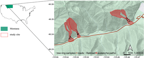
Table 1. Topographic characteristics of all avalanche paths.
Figure 2. General workflow of classification procedure from data processing to final vegetation classification.
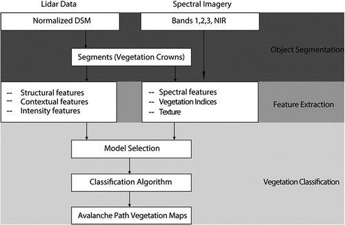
Table 2. Class aggregation for avalanche path return period analysis and detailed class descriptions.
Table 3. Overall accuracies and kappa values for random forest models of the combinations of spectral variables and lidar variables.
Figure 3. Example canopy height measurements from Shed 7. (a) In situ height measurements (m) of the four tallest trees in each field plot (open black circles). Contour lines represent 10-m elevation intervals. (b) Field plots with lidar measurements (m) for each plot. Note that samples outside the plots were considered in the validation procedure because their canopy extended over the plot area. (c) Field plots with the spectral imagery. (d) Relationship of measured mean height within each field plot (x-axis) against the lidar canopy height (y-axis). Colors represent the five field plots, and the larger dots symbolize the mean height for each plot. The dashed line is the linear regression line of all points (not including the mean values for each plot).
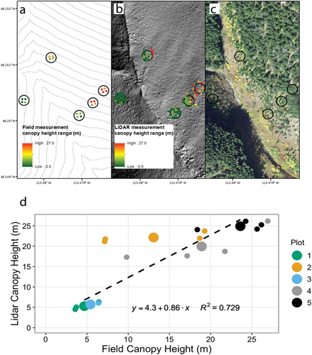
Table 4. The number of objects (points) manually identified in each vegetation class within each avalanche path.
Figure 4. The variable importance plots rank the relative importance for each variable in the best-performing random forest models (see ) for (a) model 25 (Shed 10–7), (b) model 26 (Path 1163), and (c) model 27 (Shed 7). See Table S2 for variable descriptions.
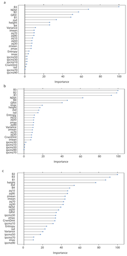
Figure 5. Modeled labeled vegetation (level 2 classes; see ) mapping results for Shed 10–7, Path 1163, and Shed 7 using a combination of spectral and lidar data. The avalanche paths are outlined with a 50-m buffer (black polygons) for context of surrounding vegetation. Note that these three paths are not all adjacent to each other ().
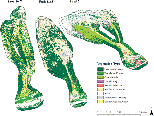
Table 5. Confusion matrices associated with the best-performing model for each individual avalanche path.
Table 6. Classification accuracies for each avalanche path using different variables or combinations of variables.
Figure 6. (a,c) Mapped return periods and (b,d) random forest model–generated vegetation classes for return interval zones for (a,b) Shed 7 and (c,d) Path 1163. The orange lines represent contour lines spaced at 10-m intervals to illustrate topography changes.
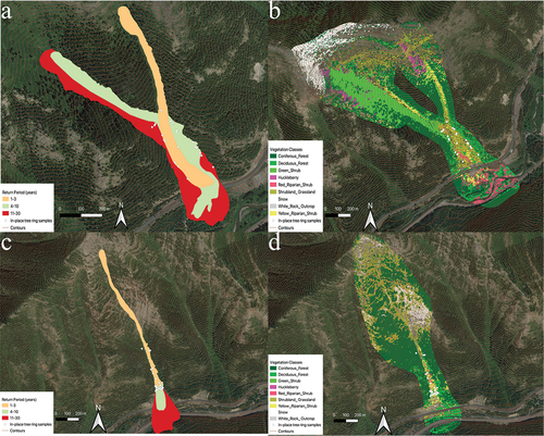
Figure 7. Proportions of each vegetation class for Shed 7 (left) and Path 1163 (right). Return interval years are represented on the x-axis. Vegetation classes are represented by color (legend on right). Note that columns do not necessarily sum to 1.0 because of classification of perennial snow in the data set.
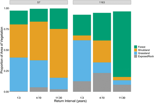
Figure 8. (a,c) Lidar-derived heights of vegetation and (b,d) raincloud plots (b,d) of tree height (m) for return intervals for (a,b) Shed 7 and (c, d) Path 1163. Raincloud plots show the individual return intervals (years) and associated tree height for each tree (points on left), box plots (center) showing the median (black horizontal line) and interquartile ranges for heights for each return interval bin, and the distribution of tree heights for each bin (shaded distribution on right). All pairwise comparisons of return intervals are significantly different in both Shed 7 and Path 1163.
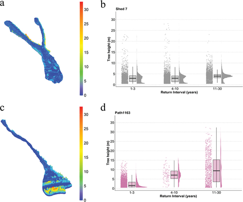
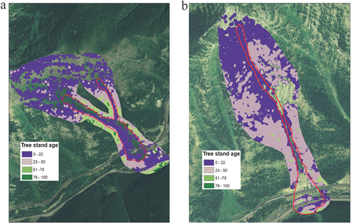
Figure 9. Tree stand age for (a) Shed 7 and (b) Path 1163. The red outline depicts the general outline of the avalanche path. The areas without color associated with a tree stand age represent areas without vegetation classified as forested areas in this study (see for classification).