Forest damage and its braking effect on the extreme snow avalanche on Mt. Nodanishoji, Japan, in 2021

Figures & data

Figure 1. Topographic map of the avalanche starting and run-out zones on Mt. Nodanishoji. The starting zones of N- and S-avalanches are shown by the red dashed ellipses. The green hatched areas and the yellow areas indicate the cedar forest and the deciduous broad-leaved forest, respectively. The red dots indicate the observed reach of the avalanche, and the red rectangle and triangles in the run-out zone are the investigation plot of a cedar forest and a row of unbroken cedar trees, respectively. Each small red line represents a fallen tree. This figure was prepared by editing the maps of the Geospatial Information Authority of Japan (GSI).

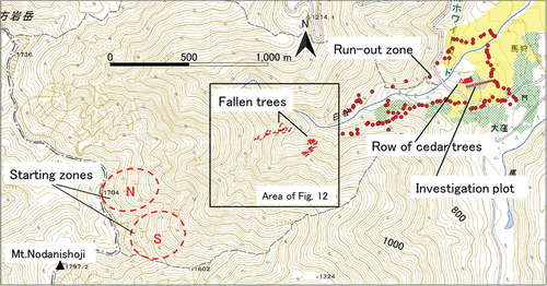
Figure 2. Aerial view of the avalanche starting and run-out zones on Mt. Nodanishoji. The white arrows in (a) indicate the starting zones of N- and S-avalanches, respectively. The red arrows are the principal direction of avalanche flow.

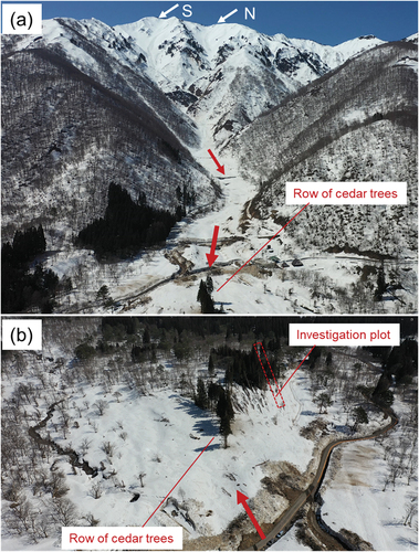
Figure 3. Avalanche damage to cedar forest in the run-out zone in 2021. The arrows in the right photo indicate the avalanche starting zones.

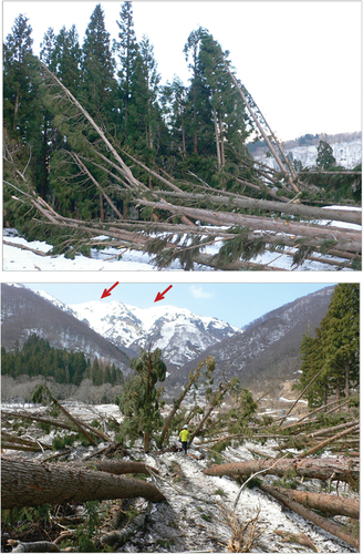
Figure 4. Measured quantities in the cedar forest.

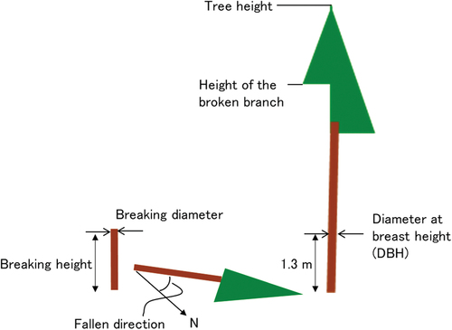
Table 1. Damage status and measurement items.

Items		Tree height	Diameter at breast height	Height of the broken branch	Breaking height	Breaking diameter	Fallen direction
Upright tree	Uninjured	○	○	—	—	—	—
	Broken branch	○	○	○	—	—	—
Leaning		○	○	○	—	—	○
Uprooted		○	○	—	—	—	○
Fallen trunk with stump		○	—	—	○	○	○
Stump without fallen trunk		—	△	—	○	○	—
Fallen trunk without stump		—	—	—	—	○	○

Note: The circles represent items that were measured, and the triangle represents one that was measured if possible.

Figure 5. A cedar stand with the bark rubbed away by the avalanche.

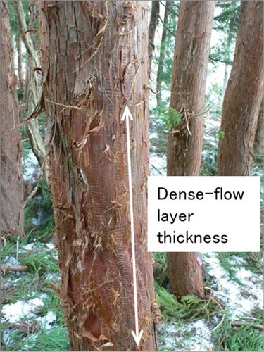
Figure 6. (a) Schematic of load on trunks from an avalanche. (b) The relationship between tree height and height of the avalanche.

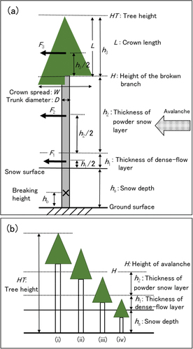
Figure 7. Cedar trees and their damage status in the investigation plot.

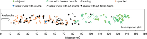
Figure 8. The levels of the peeled bark of cedar trees. The dotted lines indicate the mean value of each level.

Figure 9. The height of the broken branches. Tree height is also shown for comparison. H = height of powder snow layer; h_s + h₁ = height of dense-snow layer; h_s = height of snow.

Figure 10. (a) The breaking diameter and DBH of leaning and upright trees. (b) The breaking height of the trunks. Height of snow estimated from the level of the peeled bark is also shown for comparison. Note: We counted twenty-seven stumps without fallen trunks but only twenty-six are shown because we could not access one stump and obtained no data on its tree.

Figure 11. Avalanche velocities estimated from the bending stress of broken trunks (×). The range of 10 percent decrease is expressed by each error bar. The velocities required to break the upright trees at the ground level are also shown (○).

Figure 12. Simulation results with bed friction angle (δ) of 13° for the (a) N-avalanche and (b) S-avalanche, respectively. The extent of an avalanche with a thickness of >0.05 m is shown by the blue at 20 to 40 seconds after starting. Each red cross represents the position of a fallen tree. The results with δ of 12° and 14° are similar. The area shown in this figure is indicated in the map in Figure 1

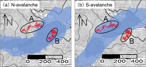
Figure 13. Variations in the average velocity of the avalanches. We unavoidably regarded these averages as equal to the velocities in the front of avalanches, because Titan2D cannot reproduce the velocity distribution of avalanches plausibly. The blue, black, and green lines represent the bed friction angles (δ) of 12°, 13°, and 14°, respectively. The plus marks and circles indicate the velocity at which the avalanche flowed into the investigation plot and reached the unbroken row of the cedar stands, respectively. The black dashed lines indicate 22 and 20 m s⁻¹. The red dashed line indicates 29 m s⁻¹. (a) N-avalanche and (b) S-avalanche.

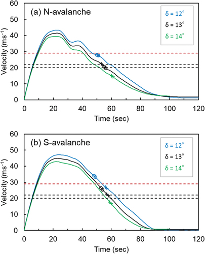
Figure 14. The simulation results at the time just before and after the avalanche reached the investigation plot (the red rectangle). The red triangles in the center are the row of unbroken cedar stands. The arrows indicate flow direction. (a) The extent of the N-avalanche at 54 and 57 seconds after starting with a bed friction angle of 13°. (b) The extent of the S-avalanche at 54 and 58 seconds after starting with a bed friction angle of 13°.

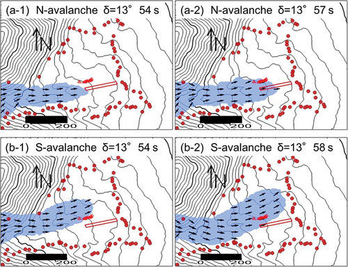
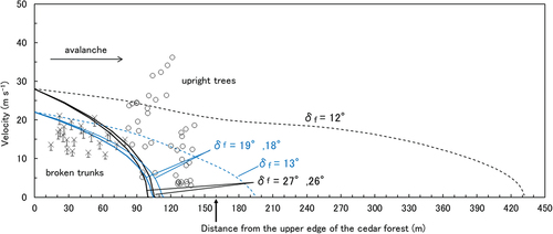
Figure 15. (a) The run-out zone of the avalanche simulations without forest. The blue area shows the extent of an avalanche with a thickness of >0.05 m. The red dots represent the observed avalanche reach. (a-1) and (a-2) are the results of N-avalanche simulations with bed friction angle (δ) of 12° and 13°, respectively, for the entire area assuming no forest. (a-3) and (a-4) are the results of S-avalanche simulations with δ of 13° and 14°, respectively, for the entire area. (b) The run-out zone of the avalanche simulations with cedar forest (the hatched areas). (b-1) and (b-2) are the results of N-avalanche simulations with δ of 12° and 13°, respectively, in the nonforested area and with δ_f of 27° and 19°, respectively, in the cedar forest. (b-3) and (b-4) are the results of S-avalanche simulations with δ of 13° in the nonforested area and with δ_f of 27° and 19°, respectively, in the cedar forest.

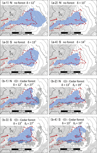
Figure 16. Comparison between the simulated velocity with bed friction angles of 27°/26° and 19°/18° (black and blue solid lines) and 12° and 13° (dashed black and blue lines). Velocities estimated from the bending stress of broken trunks (×) and the velocities required to break the upright trees at the ground level (○) are also shown for comparison. Each error bar expresses the range of a 10 percent decrease. The end of the investigation plot is shown by the arrow (↑).