
Figures & data
Figure 1. General flowchart of predicting MCF7 growth through data assimilation. (a) MCF7 breast cancer cells are grown and treated with varying doses of doxorubicin. Fluorescent microscopy is used to gather images every four hours which are converted into cell density maps. (b) A two-subpopulation model is used to describe the spatial and temporal development of MCF7 cells. (c) The model is calibrated on the cell density maps, yielding parameter values for each individual pixel. (d) We use a data assimilation pipeline consisting of successive short-term predictions guided by serial measurements. e. Cell density maps and bulk cell counts (i.e., total cell count across the entire well) are predicted at weekly intervals.
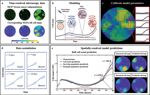
Table 1. List of model parameters.
Figure 2. Predicting MCF7 cell growth and response to doxorubicin through leave-one-out data assimilation-prediction pipeline. (a) Out of six replicates treated with similar doxorubicin doses, five are selected to form the training set and fully calibrated. Their parameter sets are averaged into parameter set Ptraining. the post-treatment data on the left-out replicate are a priori “hidden”. (b) for the replicate in the testing set, the data at the time of the treatment are used to run the model forward with parameter set Ptraining, thereby yielding a first prediction. (c) After one week, the model is informed by the data collected during this timeframe and calibrated accordingly, thereby yielding parameter set Pmeasure. (d) to predict tumor cell dynamics over the subsequent week, we first estimate the new values of the model parameters based on the degree of similarity between the tumor cell dynamics in each pixel of the replicate in the testing set and all the pixels in the training set. This comparison yields Ptraining, which we combine with Pmeasure to obtain the estimated parameter values for model prediction (i.e., Pprediction). The green shaded regions in panels b-d represent the bootstrap interquartile range of the predictions, around the dashed line representing the bootstrapped mean prediction.
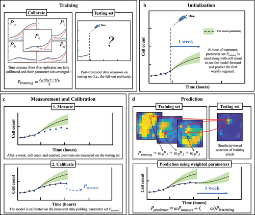
Figure 3. MCF7 breast cancer cells at various time points and treated with 10, 100 and 300 nM of Doxorubicin. Data show that low (10 nM) and high (300 nM) doses do not generate significant spatial heterogeneity post treatment, as opposed to a medium dosage where clusters of highly proliferating cells are responsible for uneven cell distribution after approximately two weeks of growth. Corresponding MATLAB tumor cell density maps can be seen on the last column.
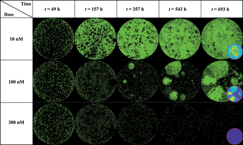
Figure 4. Model calibrations for representative replicates of MCF7 cells treated with varying doses of doxorubicin after 48 hours of growth. Measured bulk cell counts (gray circles) are shown along with the model’s estimates of the surviving (red), damaged (blue) and total (black) populations and their respective precisions. For clearer visualization, only one out of four data points are shown. The vertical dashed line represents the time of delivery of doxorubicin.
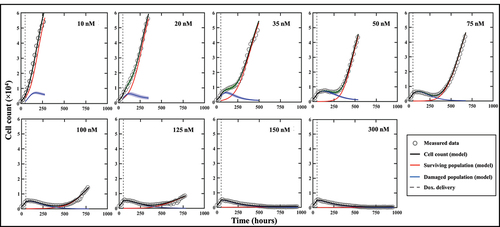
Figure 5. Spatial calibration of the two-subpopulation model on a replicate treated with 100 nM of doxorubicin. a. Bulk cell counts obtained for the global calibration of the model to the whole time course of microscopy measurements collected for the replicate, including the model’s estimate of the surviving, damaged, and total population cell counts. The calibration precision is shown on all three populations via the shaded areas. b. Our model is calibrated to fit the time course on each pixel of the well, thereby capturing the spatial heterogeneity of the tumor cell population dynamics. The cell density map is shown superimposed on the corresponding cell microscopy image, taken at the final time point (t = 782 h). The plots on the right illustrate the local counts of total, surviving, and damaged cells for three representative pixels exhibiting different temporal dynamics.
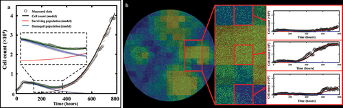
Figure 6. Spatial calibration of the two-phenotype model on a replicate treated with 35 nM of doxorubicin. (a) Bulk model calibration providing the model’s estimate of the surviving, damaged, and total population. The calibration precision is shown on all three populations (b) Cell map at final time point along with model calibration on an individual pixel at final time point (t = 497 h). (c) Distributions of each six post-treatment model parameters for pixel (6,11). The largest spreads are found on kd, gd and γd, indicative of a greater uncertainty on the estimate of the damaged population as reflected by its larger shaded area on panel a.

Figure 7. Model predictions of bulk cell count on representative replicates of MCF7 subpopulations treated with varying doses of doxorubicin after 48 hours of growth. Measured bulk cell count (gray circles) is shown along with the model’s predictions of the surviving (red), damaged (blue) and total (black) populations as well as their respective precisions. The predictions are performed on weekly segments indicated by the gray dashed lines. Our prediction pipeline is able to successfully forecast the total cell count of treated MCF7 colonies on weekly segments. For clearer visualization, only one out of four data points are shown.
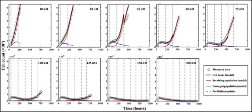
Figure 8. Spatiotemporal prediction of cell dynamics on a replicate treated with 100 nM of doxorubicin. (a) Prediction of bulk cell count. The prediction is performed on weekly segments and updated by measurements indicated by the vertical black dashed lines. (b) Comparisons between our model’s predictions of cell distribution and the map measured through microscopy at the time points indicated by the vertical dashed lines in panel A. The main patterns of heterogeneous cell distribution following doxorubicin treatment are successfully captured through data assimilation.
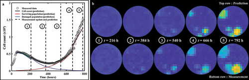
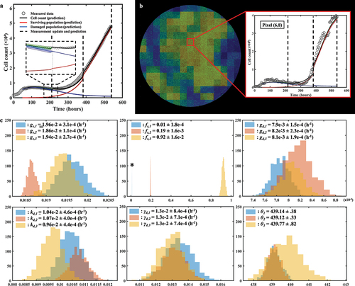
Figure 9. Parameter distributions of consecutive predictions following weekly data assimilation. (a) Prediction of bulk cell count on a replicate treated with 50 nM of doxorubicin. (b) Prediction of cell count on pixel (6,8). (c) Bootstrapped parameter distributions for model predictions on pixel (6,8), showing the shift in the mean value and variance of the post-treatment parameters between each weekly timeframe. The distribution for the first weekly segment of parameter fs is indicated by a star as it is so narrow and may be difficult to see. The changes in the width of the parameter distributions is representative of changes in the uncertainty in the parameter value, which emanate from the quality of the model fit in the preceding weeks as well as from the wide variety of parameter values in similar pixels in the training set. The changes in the mean value point toward changes in the overall dynamics identified by the model as more data is progressively assimilated on a weekly basis.
Supplementary figures.docx
Download MS Word (242.7 KB)Data availability statement
Publicly available datasets were analyzed in his study. This data can be found here: https://doi.org/10.5281/zenodo.6973776.