Monitoring forest decline through remote sensing time series analysis

Figures & data

Figure 1. Study sites (map background: French Geographic National Institute (IGN)).

Figure 2. Spring greenness (SG) values for the study period and the SG trend, for a single pixel.

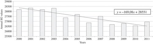
Figure 3. BFAST decomposition of NDVI time series from 2000 to 2011 for a single pixel containing coniferous stands. Yt = original time series, St = seasonal component, Tt = trend component, and et = remainder component.

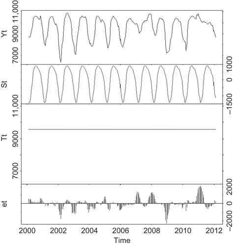
Figure 4. BFAST decomposition of NDVI time series for the 2000–2011 period for a single pixel. The date of the most important breakpoint is indicated by the dashed vertical line.

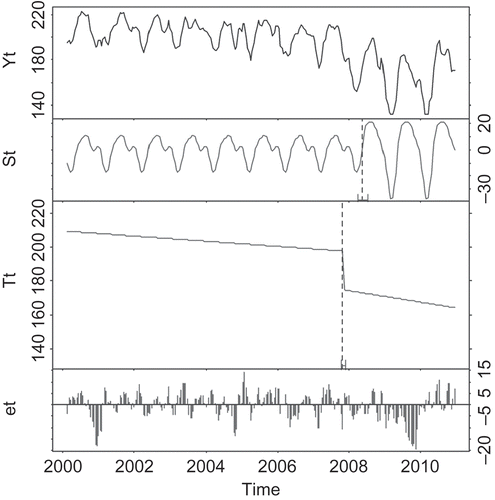
Figure 5. Sampling design used for each field plot.

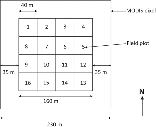
Table 1. Typology of the health status of silver fir as a function of the extent of the symptoms of decline of the crown and/or the recovery process

Signs of degradation	Recovery process	Mature tree state
None	None	Normal state HEAlthy tree
Low  Presence of significant mortality in the crown, but dense foliage ; or low density foliage, but mortality limited to A3	Low  Absence or a few of vigorous epicormic branches	Deviation to normal state STRessed tree
	Dominant  Presence of many epicormic branches	Return to normal state RESilient tree
Significant  Low density foliage and mortality not limited to A3	Low  Absence or a few of vigorous epicormic branches	Impossible return to normal DEAd or dying tree

Figure 6. Illustrations of the four main ARCHI type: (a) HEAlthy tree, (b) STRessed tree, (c) RESilient tree, and (d) DEAd or dying tree.

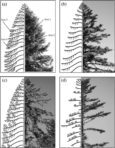
Table 2. Level and type of observations recorded with the ARCHI method

Observation level	Nature of the observations
Whole tree	Mortality
	Presence and vigor of epicormic branches
	Presence of a second crown
Upper crown	Presence of mortality. Symptoms of degradation
	Foliage density and level of visibility of the trunk
	Presence – abundance and vigor of epicormic branches
Axes (Al to A4)	Presence of mortality
	Loss of branches
	Abnormal coloration, foliar deficit Decline or regrowth

Figure 7. Scatterplots of the standardized slope of the trends processed using spring greenness (x-axis) and BFAST (y-axis) for (a) the whole series and for (b) for spring dates only.

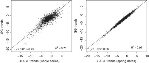
Figure 8. Map of trends (a) produced with the spring greenness method and (b) with the BFAST method (site 1).

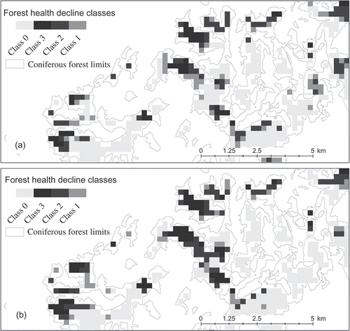
Table 3. Contingency matrices between classes of (a) SG and BFAST trends for the whole series and (b) SG and BFAST trends for spring dates only

(a)	BFAST trend classes
SG trend classes	0	1	2	3
0	93.7%	5.2%	1.1%	0%
1	72.1%	21.5%	6.4%	0%
2	32%	31.8%	34.6%	1.6%
3	0.6%	3.2%	36.5%	59.6%
(b)	BFAST trend classes (spring dates)
SG trend classes	0	1	2	3
0	93.1%	6.7%	0.2%	0%
1	8.4%	67.8%	23.7%	0%
2	0%	7.4%	86.1%	6.5%
3	0%	0%	1.9%	98.1%

Figure 9. Barplots of (left) annual count of negative breakpoints and (right) means of negative breakpoints with standard deviation.

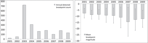
Figure 10. Proportion of main ARCHI types in the 27 pixels observed at ground level.

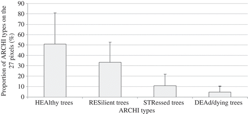
Figure 11. Relations between proportions of the main ARCHI types and measured spring greenness trends in the period 2000–2011.

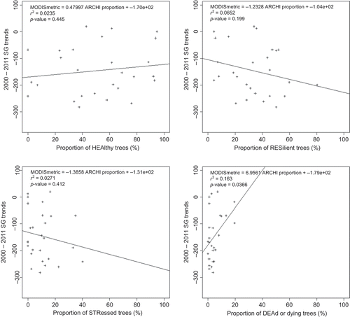
Figure 12. Variations in r ² values between spring greenness and the proportion of main ARCHI types as a function of the year.

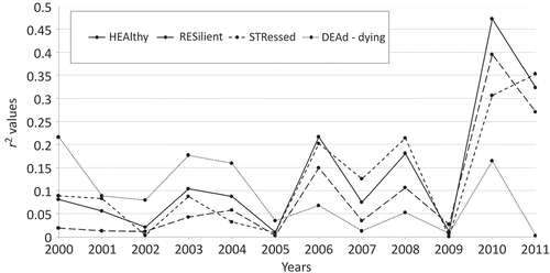
Figure 13. Relationships between the proportions of the main ARCHI types and spring greenness values in 2010.

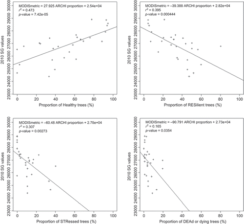
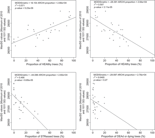
Figure 14. Relationships between the proportion of ARCHI types and the MaxSG indicator (maximum of SG values of years 2010 and 2011).

Table 4. R ² values of the relationships between MODIS time series-derived metrics and ARCHI proportions of the four ARCHI type with p-values (*p < 0.05, **p < 0.01, ***p < 0.001)

MODIS time series-derived metric	HEAlthy tree proportions	RESilient tree proportions	STRessed tree proportions	DEAd or dying tree proportions
2000–2011 SG trends	0.02	0.06	0.03	0.16*
	(0.44)	(0.20)	(0.41)	(0,04)
Annual SG values (year 2010)	0.47***	0.39***	0.31**	0.16*
	(<0.001)	(<0.001)	(<0.01)	(0,04)
MaxSG indicator values: maximum of SG values (years 2010 and 2011)	0.57***(<0.001)	0.51***(<0.001)	0.47***(<0.001)	0.05(0,27)