Expansion of LISS III swath using AWiFS wider swath data and contourlet coefficients learning

Figures & data

Table 1. Resourcesat-2 AWiFS and LISS III sensors’ characteristics.

	AWiFS	LISS III
Spatial resolution	56 m	23.5 m
Swath width	740 km	140 km
Spectral bands ()	B2: 0.52–0.59	B2: 0.52–0.59
	B3: 0.62–0.68	B3: 0.62–0.68
	B4: 0.77–0.86	B4: 0.77–0.86
	B5: 1.55–1.70	B5:1.55–1.70
Temporal resolution	(Revisit) 5 days	24 days

Figure 1. Overlapped LISS III at the center portion of full AWiFS scene in simultaneous acquisition.

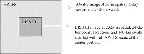
Figure 2. Nonsubsampled contourlet transform. (a) Nonsubsampled filter banks structure that implements the NSCT. (b) Frequency partitioning which is obtained with the filter banks shown in (a). Source: Da Cunha, Zhou, and Do (2006). © IEEE. Reproduced by permission of IEEE.

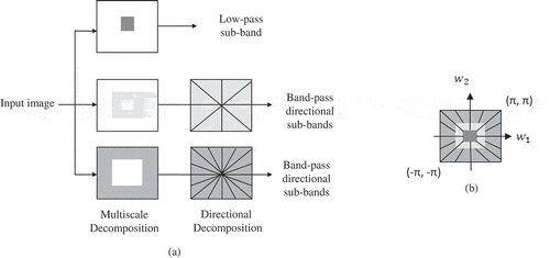
Figure 3. Training phase of the overlapping regions of AWiFS and LISS III images over NSCT domain.

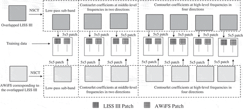
Figure 4. Prediction of AWiFS data in the nonoverlapping region at LISS III spatial resolution using the overlapping regions of LISS III and AWiFS as prior knowledge.

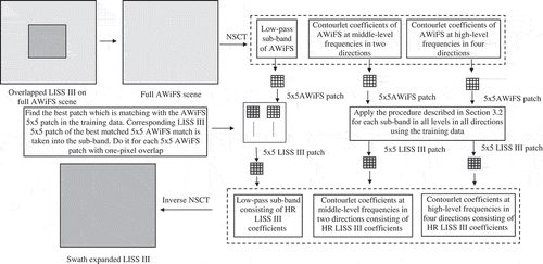
Figure 5. Swath-expanded LISS III (in green-red-near-infrared (NIR) false color composition) using SVR and the proposed CCL. (a) LISS III overlapped at the center of full AWiFS scene (input image). (b) Swath-expanded LISS III using SVR Zhang and Huang (2013) method. (c) Swath-expanded LISS III using CCL (proposed method). (d) Original LISS III.

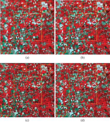
Table 2. Quantitative comparison between predicted and actual reflectance for the experimental data-set: 1.

Method	Computational time (in hours per band)	SSIM				RMSE				SAM
		B2	B3	B4	B5	B2	B3	B4	B5
CCL (proposed method)	4	0.9494	0.9344	0.9255	0.9494	0.0062	0.0108	0.0120	0.0071	1.8753
SVR (Zhang and Huang 2013)	16	0.9385	0.9250	0.9058	0.9316	0.0069	0.0118	0.01309	0.0084	1.8942

Note: Bold indicates the proposed method is superior in every quality parameter of the Table 2 when compared to an SVR method.

Figure 6. Scatter plots between the predicted and actual reflectance values of SVR and the proposed CCL methods (where scale factor is 1000).

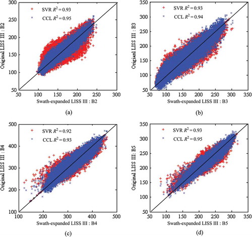
Figure 7. Swath-expanded LISS III (in green-red-NIR false color composition) using SVR and the proposed CCL. (a) LISS III overlapped at the center of full AWiFS scene (input image). (b) Swath-expanded LISS III using SVR Zhang and Huang (2013) method. (c) Swath-expanded LISS III using CCL (proposed method). (d) Original LISS III.

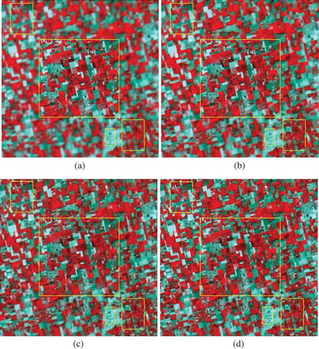
Table 3. Quantitative comparison between predicted and actual reflectance for the experimental data-set: 2.

Method	Computational time (in hours per band)	SSIM				RMSE				SAM
		B2	B3	B4	B5	B2	B3	B4	B5
CCL (proposed method)	4	0.9508	0.9418	0.9325	0.9519	0.0064	0.0113	0.0125	0.0071	1.4786
SVR (Zhang and Huang 2013)	16	0.9346	0.9217	0.9076	0.9308	0.0074	0.0127	0.0141	0.0082	1.5251

Note: Bold indicates the proposed method is superior in every quality parameter of the Table 3 when compared to an SVR method.

Figure 8. Scatter plots between predicted and actual reflectance values of SVR and the proposed CCL methods (where scale factor is 1000).

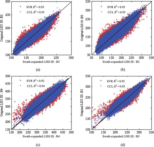
Figure 9. Relative spectral response (RSR) of Resourcesat-2 AWiFS and LISS III sensors.

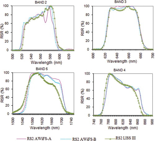
Table 4. Techniques to normalize the differences between AWiFS and LISS III sensor data.

Difference	Techniques to reduce the difference
Atmospheric effect	AWiFS and LISS III images have similar atmospheric effects in the overlapping region because they are acquired at the same time.
Sun elevation angle Sun azimuth angle Sensor elevation angle Sensor azimuth angle	Because the images of AWiFS sensor are across ± 24.3° from nadir, its overlapping and nonoverlapping regions with LISS III have the potential of being impacted by bidirectional reflectance distribution function (BRDF) phenomena. These BRDF biases can be corrected with reflectance correction factor with respect to the view zenith angle (Walthall et al. 1985; Goward et al. 2012; Srivastava et al. 2014).
Spectral bandwidth	Although AWiFS and LISS III sensors have same spectral bandwidths, they have different relative spectral response (RSR) as shown in Figure 9. So the AWiFS reflectance was normalized to LISS III reflectance by the procedure described in Chander, Coan, and Scaramuzza (2008).
Spatial resolution	The nonoverlapping region of AWiFS with LISS III is enhanced to LISS III spatial resolution using CCL (proposed method).

Da Cunha, A. L., J. Zhou, and M. N. Do. 2006. “The Nonsubsampled Contourlet Transform: Theory, Design, and Applications.” IEEE Transactions on Image Processing 15: 3089–3101. doi:10.1109/TIP.2006.877507.

 PubMed Web of Science ®Google Scholar

Zhang, H., and B. Huang. 2013. “Support Vector Regression-Based Downscaling for Intercalibration of Multiresolution Satellite Images.” IEEE Transactions on Geoscience and Remote Sensing 51: 1114–1123. doi:10.1109/TGRS.2013.2243736.

 Web of Science ®Google Scholar

Walthall, C. L., J. M. Norman, J. M. Welles, G. Campbell, and B. L. Blad. 1985. “Simple Equation to Approximate the Bidirectional Reflectance from Vegetative Canopies and Bare Soil Surfaces.” Applied Optics 24: 383–387. doi:10.1364/AO.24.000383.

 PubMed Web of Science ®Google Scholar

Goward, S. N., G. Chander, M. Pagnutti, A. Marx, R. Ryan, N. Thomas, and R. Tetrault. 2012. “Complementarity of Resourcesat-1 AWiFS and Landsat TM/ETM+ Sensors.” Remote Sensing of Environment 123: 41–56. doi:10.1016/j.rse.2012.03.002.

 Web of Science ®Google Scholar

Srivastava, P. K., D. Han, M. A. Rico-Ramirez, M. Bray, T. Islam, M. Gupta, and Q. Dai. 2014. “Estimation of Land Surface Temperature from Atmospherically Corrected LANDSAT TM Image Using 6S and NCEP Global Reanalysis Product.” Environmental Earth Sciences. doi:10.1007/s12665-014-3388-1.

 Web of Science ®Google Scholar

Chander, G., M. J. Coan, and P. L. Scaramuzza. 2008. “Evaluation and Comparison of the IRS-P6 and the Landsat Sensors.” IEEE Transactions on Geoscience and Remote Sensing 46: 209–221. doi:10.1109/TGRS.2007.907426.

 Web of Science ®Google Scholar