Figures & data
Figure 1. Eight cities in the Pearl River Delta, along with the NSL characteristics.
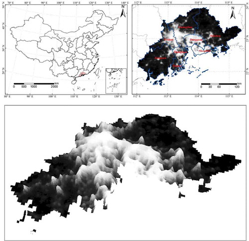
Table 1. Landsat TM/ETM+ images of eight cities in the Pearl River Delta.
Figure 2. Technical approach used in the study.
Figure 3. Deriving the topographic maps using the neighborhood statistics analysis method. Figure ‘a’–‘d’ shows the original DMSP/OLS imageries of the city of Guangzhou in 1996, 2000, 2005, and 2009, respectively; Figure ‘e’–‘h’ shows the corresponding topographic maps.
Figure 4. Extracting the built-up urban areas in HVR. Figure ‘a’–‘d’ represents the three classified areas (transition zones (TZ); built-up urban lands (BL); and non-built-up urban lands (NBL)) in 1996, 2000, 2005, and 2009, respectively; Figure ‘e’–‘h’ represents the extracted built-up areas in HVR.
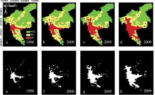
Figure 5. Extracting the built-up urban areas hidden in the transition zones. Figure ‘a’–‘d’ represents subtracted results that are derived by subtracting the output raster of minimum-NSA in the 5 × 5 cell window from that in the 3 × 3 cell window in 1996, 2000, 2005, and 2009, respectively; Figure ‘e’–‘h’ represents the extracted built-up urban areas in the transition zones.
Figure 6. The entire built-up urban areas of Guangzhou extracted from NSL in 1996, 2000, 2005, and 2009.
Figure 7. The built-up urban areas of eight cities in the Pearl River Delta of southern China in 1996, 2000, 2005, and 2009. Figure ‘a’–‘d’ represents the original DMSP/OLS NSL imageries; Figure ‘e’–‘h’ represents the Landsat TM/ETM+-extracted built-up urban areas; Figure ‘i’–‘l’ represents the NSL-extracted built-up urban areas using the global-fixed threshold method; Figure ‘m’–‘p’ represents the NSL-extracted built-up urban areas using the local-optimized threshold method; Figure ‘q’–‘t’ represents the NSL-extracted built-up urban areas using the proposed NSA method.
Table 2. Validation accuracies of DMSP/OLS NSL-extracted built-up urban areas using the confusion matrix method in Matab.
Table 3. Definition of the landscape indices.
Table 4. Comparison of the landscape indices between DMSP/OLS NSL-mapped built-up urban areas with those from Landsat TM/ETM+ imageries.
Figure 8. Comparison of the landscape indices of DMSP/OLS NSA-derived built-up urban areas with those of Landsat TM/ETM+ images. (a) The total area (CA); (b) the landscape shape index (LSI); (c) the contiguity index (CONTIG); and (d) the perimeter area ratio (PARA).
Figure 9. Scatter diagrams between the total NSL of NSA-extracted built-up urban areas and statistical urban population.
Figure A1. Maximum/minimum neighborhood statistics analysis for single cells and for the entire data set.
Figure A2. Technical approach for extracting built-up urban areas from Landsat TM/ETM+ images.