Figures & data
Table 1. Input variables and reference data information.
Figure 1. The process flow of the research.
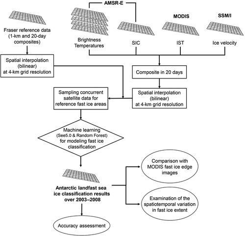
Table 2. Accuracy assessment results for decision trees using the test data-set.
Table 3. Accuracy assessment results for random forest using the test data-set.
Figure 2. Box plots of the producer’s accuracy and user’s accuracy for quantitative examination of the fast ice mapping results of (a) decision trees and (b) random forest. For full color versions of the figures in this paper, please see the online version.
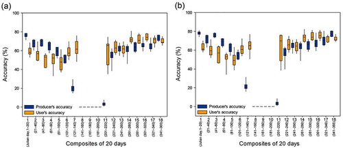
Table 4. Attribute usage of the decision trees model.
Table 5. Mean decrease accuracy calculated using out-of-bag data when a variable was permuted in random forest. The greater the decrease in accuracy, the more contributing the variable was.
Figure 3. Comparison of fast ice mapping results by model with the 250-m MODIS images during the periods of relatively stable fast ice around (a) Mertz and (b) Abbot Ice Shelf in the East and West Antarctica, respectively. The lines in (a) and (b) indicate fast ice edges delineated from the MODIS images based on visual interpretation. Decision tree results are shown in (c) and (d), while random forest results are in (e) and (f). MODIS images with the maximum fast ice cover were used as background images in (a) and (b).
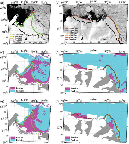
Figure 4. Comparison of fast ice mapping results by model with the 250-m MODIS images during the periods of rapidly changing fast ice around (a) Mertz and (b) Abbot Ice Shelf in the East and West Antarctica, respectively. The lines in (a) and (b) indicate fast ice edges delineated from the MODIS images based on visual interpretation. Decision tree results are shown in (c) and (d), while random forest results are in (e) and (f). MODIS images with the maximum fast ice cover were used as background images in (a) and (b).
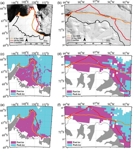
Figure 5. Fast ice maps using random forest in 2003 for (a) composite 5 (81–100 Julian days) and (b) composite 13 (241–260 Julian days). Magenta areas represent fast ice in the Antarctic, and hatched areas with gray color indicate that MODIS IST was not available for the composite.
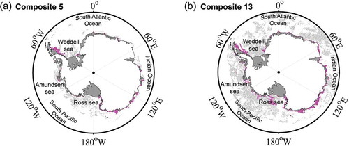
Figure 6. (a) Temporal variation of the availability of MODIS IST data in the East and West Antarctic regions. (b) The ratio of the IST coverage in the West Antarctic (WA) relative to the East Antarctic (EA) in percentage. (c) Box plot of the IST coverage in percentage by composite.
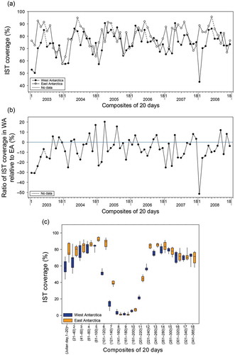
Figure 7. Temporal variation of fast ice areas in the East and West Antarctic. Due to the lack of the input data during the Australian winter season, composites 6–12 for each year were not available.
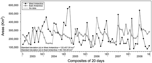
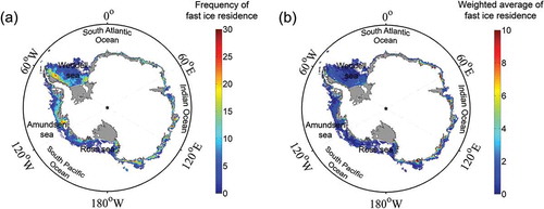
Figure 8. Temporal variation of fast ice in the Antarctic using (a) the simple counting approach and (b) the weighted average approach.