Land change attribution based on Landsat time series and integration of ancillary disturbance data in the Athabasca oil sands region of Canada

Figures & data

Figure 1. Overview outlining the key processing steps and datasets used in the analysis.

Figure 2. Area of interest shown in grey.

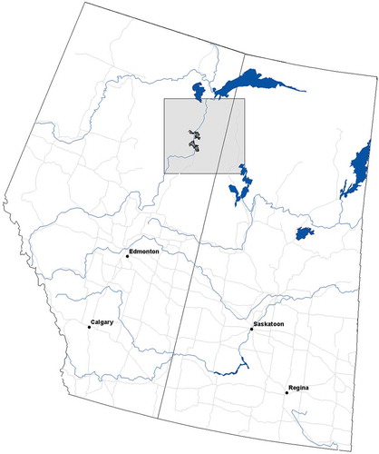
Table 1. Change classes and rulesets used for change type classification.

Class	Ruleset
Forest harvest	Abrupt change segment associated with ABMI_HF harvest polygon detected year and post-disturbance spectral response >50% bare membership and post-disturbance land cover was not needleleaf, broadleaf, or mixed forest. Pre-disturbance land cover was either needleleaf, broadleaf, or mixed forest
Fire	(1) Abrupt change segment associated with NCLFD fire polygon and post-disturbance spectral response with >50% fire membership and post-disturbance land cover was not needleleaf, broadleaf, or mixed forest. (2) Abrupt change segment with post-disturbance spectral response >80% fire membership and post-disturbance land cover was not needleleaf, broadleaf, or mixed forest. This is a conservative rule that accounts for fires missed in the NCLFD
Insect damage	Gradual change segment and insect-damage membership > bare, flood, or fire memberships and pre-disturbance forest needleleaf, broadleaf, or mixed-forest membership was >70%
Flooding	Segments where post-disturbance water membership was greater than 60% for more than 2-years post-disturbance
Regeneration	Temporal segments that increased their forest fraction by 20% over at least 3 years and the final forest fraction was greater than 20% following disturbance. To account for disturbances prior to 1985, this rule was applied to the first segment in the time series
Surface mining	Segments that had a harvest-spectral membership post-disturbance >50% and were associated with the crude mining footprint mask for the year
Abrupt disturbance without regeneration	Changes that occurred rapidly (≤2 years), were not followed by regeneration as per criteria for regeneration, and were not previously classified to a change type. This class was commonly associated with mining or exploration activities such as roads, pipelines, well pads, etc.
Gradual disturbance without regeneration	Changes that occurred gradually (>2 years), were not followed by regeneration as per criteria for regeneration, and were not previously classified to a change type
Abrupt disturbance with regeneration	Changes that occurred rapidly (≤2 years) with regeneration as per criteria for regeneration, and were not previously classified to a change type
Gradual disturbance with regeneration	Changes that occurred gradually (>2 years) with regeneration as per criteria for regeneration, and were not previously classified to a change type
Spectral variability likely associated with wetlands	Areas of change where the pixel was classified as wetland more than four times in the time series
Unclassified	Changes with small magnitude that were not assigned to another class. This was largely due to commission error and not included as change
Haze	Segments identified as change with a haze membership greater than 80% and not associated with a harvest or fire disturbance. These segments were not considered change

Figure 3. Example time series for harvesting in 1989 and fire in 2011 (A–B) and insect damage (C–D). Cloud- and shadow-screened time series are shown as asterisks. Blue line represents average value in each year. Sub-trend time series results (red line) from the average values shown as the black line.

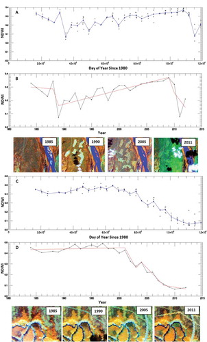
Table 2. Change/no-change error matrix.

	Reference
	Change	No-change
Change	193	20
No-change	9	37
Overall accuracy %		89

Table 3. Change type error matrix.

		Reference
		1	2	3	4	5	6	7	8	9	10	11	12
Forest harvest	1	20	0	0	0	0	0	0	0	0	0	0	0
Forest fire	2	0	20	0	0	0	0	0	0	0	0	0	0
Insect damage	3	0	2	15	0	0	0	0	0	0	0	3	0
Flooding	4	0	0	0	20	0	0	0	0	0	0	0	0
Forest regeneration	5	0	0	0	0	20	0	0	0	0	0	0	1
Surface mining	6	0	0	0	0	0	20	0	0	0	0	0	0
Abrupt dist. no regen.	7	1	0	0	0	0	2	15	0	0	0	1	0
Gradual dist. no regen.	8	0	0	0	0	0	0	2	12	0	0	7	1
Abrupt dist. regen.	9	4	0	0	0	0	0	0	1	11	0	2	2
Gradual dist. regen.	10	1	0	1	0	0	0	0	0	0	7	9	2
Wetland variability	11	0	0	0	0	0	0	1	0	0	0	18	0
No Change	12	0	0	1	0	3	0	0	0	0	0	0	35
Producer’s accuracy %		77	91	88	100	87	91	83	92	100	100	45	85
User’s accuracy %		100	100	75	100	95	100	79	55	55	35	95	90
Ave. prod. and user’s %		88	95	82	100	91	95	81	73	78	68	70	88
Overall accuracy %		82

Table 4. Change error timing estimates by change type.

	Error start year					Error end year
Change type	Abs mean Std. Dev. 90%ile			Max	Abs mean	Dev. 90%ile		Max
Forest harvest	0.30	0.92	1	4	0.2	0.89	0	4
Fire	0.10	0.31	0	1	0.1	0.22	0	1
Insect damage	0.25	0.64	1	2	1.1	1.74	3	6
Flooding	3.00	2.87	7	9	1.9	1.77	3	6
Surface mining	1.05	1.76	4	6	0.5	0.61	1	2
Abrupt dist. no regen.	0.11	0.32	1	1	0.0	0.00	0	0
Gradual dist. no regen.	0.32	0.89	1	3	0.2	0.40	1	1
Abrupt dist. regen.	0.10	0.31	0	1	0.2	0.41	1	1
Gradual dist. regen.	0.15	0.49	0	2	0.4	1.35	1	6
Wetland variability	0.00	0.00	0	0	0.1	0.23	0	1

*Regenaration and haze classes were not assessed as interperation in the available reference data was insufficient.

Table 5. Land-cover error matrix.

		Reference
		1	2	3	4	5	6	7	8	10
Needleleaf high density	1	53	4	1	0	2	6	1	1	0
Needleleaf low density	2	11	56	0	2	10	8	4	4	3
Mixed forest	3	1	1	13	0	1	4	0	1	0
Broadleaf	4	2	5	3	41	9	0	1	0	0
Shrub	5	1	2	3	3	78	20	6	0	0
Low vegetation cover	6	2	4	0	0	1	39	4	0	0
Barren	7	4	4	1	0	0	3	38	2	3
Wetland	8	0	0	0	1	6	2	0	16	0
Water	10	3	1	0	0	1	0	1	0	22
Producer’s accuracy %		69	73	62	87	72	48	69	67	79
User’s accuracy %		78	57	62	67	69	78	69	64	79
Ave. prod. and user’s %		73	65	62	77	71	63	69	65	79
Overall accuracy %		69

Figure 4. Summary of the change types for most recent change (A), year of most recent change (B), change severity of most recent change (C), and Landsat composite for 2012 for comparison (D).

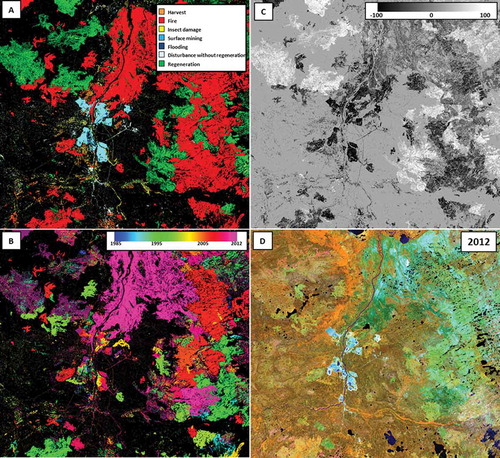
Figure 5. Trends in change type. (A) Pixel count converted to hectares and (B) Sum of forest fraction change by change type. Note the scaling for fire and the secondary axis used for regeneration to enhance interpretability. In (B), all disturbances have been multiplied by −1 and actually represent a negative forest fraction change.

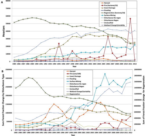
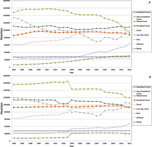
Figure 6. Trends in land cover for pixel count converted to hectares based on the original land cover (A) and the temporally filtered (B).