Environmental evaluation of MODIS-derived land units

Figures & data

Figure 1. (a) MODIS-based LUs obtained by segmenting three EVI and three second moment images (scale parameter of 15 (Bisquert, Bégué, and Deshayes 2015), superimposed to a color composition of MODIS EVI of April (R), July (G), and December (B) averaged over 2007–2011. (b) Distribution of the LUs areas. For full color versions of the figures in this paper, please see the online version.

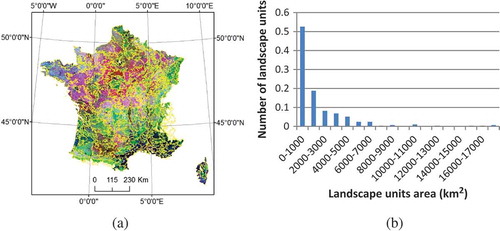
Figure 2. Environmental variables used in the explanatory analysis of the stratification: (a) average maximum temperature (Météo France; 2007–2011); (b) average minimum temperature (Météo France; 2007–2011); (c) normal annual cumulated precipitations (Joly et al. 2010); (d) elevation (GTOPO 30); (e) parent material (Van Liedekerke, Jones, and Panagos 2006). Only the nine dominant parent materials of the STU are represented for the sake of clarity; (f) CORINE land cover 2006 (European Environment Agency 2007). Only the five main (level 1) categories are  shown for the sake of clarity. The LUs map obtained in Bisquert, Bégué, and Deshayes (2015) is superposed in all cases. For full color versions of the figures in this paper, please see the online version.

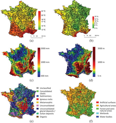
Figure 3. Pyrenean land cover map (adapted from http://www.cesbio.ups-tlse.fr/newsletter_cesbio/numero8/Vmail.html#sudouest1, accessed 10/06/2013). The fraction of the class presence is given in parenthesis. The black line corresponds to the France–Spain border. For full color versions of the figures in this paper, please see the online version.

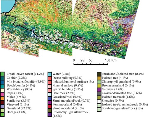
Figure 4. Scheme of the analysis performed and data used.

Figure 5. Simplified Pyrenean land cover map (see Table 2), overlaid with the stratification results obtained by Bisquert, Bégué, and Deshayes (2015), and divided in three zones (land 1: red; land 2: blue; land 3: pink) that correspond to different Landsat image acquisition dates. For full color versions of the figures in this paper, please see the online version.

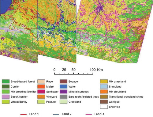
Figure 6. Example of test areas (black lines) along the boundaries (blue line) between neighboring LUs used for analyzing the boundaries quality. The legend is the same as in Figure 5. For full color versions of the figures in this paper, please see the online version.

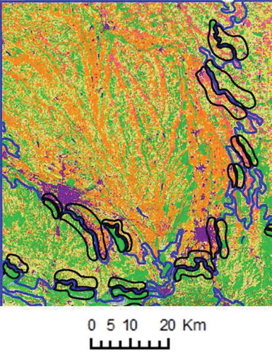
Table 1. Moran’s index calculated on the environmental quantitative variables, at national scale.

	Altitude	T_max	T_min	Precipitation
Moran’s index	0.48	0.86	0.69	0.73

Table 2. Land cover classes correspondence between the Pyrenean cover map (Figure 3) and the simplified Pyrenean cover map (Figure 5).

New land cover	Original cover
Grassland	Chlorophyll grassland
	Brown grassland
Mix grassland	Grassland/bare rock
	Chlorophyll grassland/bare rock
	Grassland/isolated tree
	Isolated tree/grassland/bare rock
Shrubland	Fern moorland
	Shrub moorland
Mix shrubland	Shrub moorland/bare rock
	Shrubland/isolated tree
	Shrubland/grassland/bare rock
Mineral surfaces	Dense building
	Industrial/mineral surface
	Mineral surface
	Sparse buildings
Bare rocks/isolated trees	Bare rock
	Isolated tree

Note: The classes that are common to both maps are not presented in the table.

Bisquert, M., A. Bégué, and M. Deshayes. 2015. “Object-Based Delineation of Homogeneous Landscape Units at Regional Scale Based on MODIS Time Series.” International Journal of Applied Earth Observation and Geoinformation 37: 72–82. doi:10.1016/j.jag.2014.10.004.

 Web of Science ®Google Scholar

Joly, D., T. Brossard, H. Cardot, J. Cavailhes, M. Hilal, and P. Wavresky. 2010. “Les Types de Climats En France, Une Construction Spatiale.” Cybergeo. doi:10.4000/cybergeo.23155.

 Google Scholar

Van Liedekerke, M., A. Jones, and P. Panagos. 2006. “ESDBv2 Raster Library-a Set of Rasters Derived from the European Soil Database Distribution v2. 0.” European Commission and the European Soil Bureau Network, CDROM, EUR, 19945.

 Google Scholar

European Environment Agency. 2007. CLC2006 Technical Guidelines, 17. http://www.eea.europa.eu/publications/technical_report_2007_17.

 Google Scholar