Integrating the multi-label land-use concept and cellular automata with the artificial neural network-based Land Transformation Model: an integrated ML-CA-LTM modeling framework

Figures & data

Figure 1. (a) mono-label classification (ml) with two land-use classes (gray and black) and (b) Multi-Label classification (ML) with cells belonging to both classes (squares split by the two colors).

Figure 2. Conceptual diagram of the ML-CA-LTM model.

Figure 3. Conversion of a vector map to a raster map with ML: (a) vector data containing polygons with land-use codes; (b) rasterizing vector data; (c) the value of each grid in raster space depends on the land-use code of the polygons which cover them.

Figure 4. Architectures of the neural network BP-MLL (in the left) and BP (in the right) showing input, hidden and output layers.

Figure 5. Processing steps of the ML-CA-LTM model. Note that the estimated label set for a given cell is fixed by a threshold which is to be optimized, as suggested by Zhang and Zhou (2006).

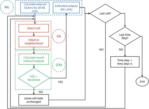
Table 1. Example of a testing set.

Observed	Observed Class				Neural output				Estimated class				Estimated
Label set	y1	y2	y3	y4	y1	y2	y3	y4	y1	y2	y3	y4	Label set
{y1, y4}	1	0	0	1	0.5	0.1	0.6	0.2	1	0	1	0	{y1, y3}
{y2, y3}	0	1	1	0	0.3	0.7	0.4	0.1	0	1	1	0	{y2, y3}
{y1, y4}	1	0	0	1	0.5	0.2	0.2	0.6	1	0	0	1	{y1, y4}
{y2}	0	1	0	0	0.2	0.8	0.1	0.6	0	1	0	1	{y2, y4}
{y1, y3}	1	0	1	0	0.9	0.3	0.2	0.1	1	0	0	0	{y1}

Note: The selected outputs, based on an optimized threshold = 0.45, are shown in bold.

Figure 6. Luxembourg and its bordering areas.

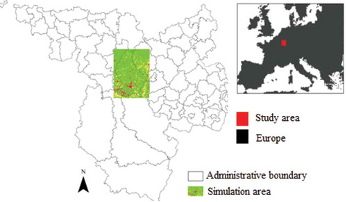
Table 2. Driving features as input of the model.

Category	Variable	Description
Physical	State_cell Y = (y1,y2,y3,y4)	Multi-label class
	X1: Slope	Slope value of cell (%)
	X2: Urban_neighbours	Amount of urban cells in the 3 × 3 Moore neighborhood
	X3: Industrial_neighbours	Amount of industrial cells in the 3 × 3 Moore neighborhood
	X4: Agriculture_neighbours	Amount of agriculture cells in the 3 × 3 Moore neighborhood
	X5: Forest_neighbours	Amount of forest cells in the 3 × 3 Moore neighborhood
	X6: Water_neighbours	Amount of water cells in the 3 × 3 Moore neighborhood
City/country distances	X7: Distance_border	Distance from cell to the border of Luxembourg country (m)
	X8: Distance_main_city1	Distance from cell to the city of Luxembourg (m)
	X9: Distance_ main_city2	Distance from cell to the city of Esch (m)
	X10: Distance_ main_city3	Distance from cell to the city of Differdange (m)
Transportation	X11: Transport_neighbours	Amount of transport cells in the 3 × 3 Moore neighborhood
	X12: Distance_bus_stations	Distance from cell to the closest bus station (m)
	X13: Distance_train_stations	Distance from cell to the closest train station (m)
	X14: Distance_highway	Distance from cell to the nearest highway access point (m)
	X15: Number_bus_station	Number of bus stations located 2 km away from cell
	X16: Number_train_station	Number of train stations located 2 km away from cell

Table 3. Multi-label land-use data in 2007.

					Observed label set
	Class				1999		2007
Label set	U	I	A	F	#	%	#	%
F	0	0	0	1	56,730	22.19	57,297	22.41
A	0	0	1	0	75,320	29.46	73,025	28.56
AF	0	0	1	1	77,330	30.24	76,777	30.03
I	0	1	0	0	1305	0.51	1282	0.50
FI	0	1	0	1	1961	0.77	2141	0.84
AI	0	1	1	0	2558	1.00	3001	1.17
AFI	0	1	1	1	2277	0.89	2609	1.02
U	1	0	0	0	3933	1.54	3796	1.48
FU	1	0	0	1	3583	1.40	3862	1.51
AU	1	0	1	0	17,024	6.66	15,565	6.09
AUF	1	0	1	1	9342	3.65	9375	3.67
IU	1	1	0	0	973	0.38	1426	0.56
FIU	1	1	0	1	795	0.31	1046	0.41
AIU	1	1	1	0	1517	0.59	2943	1.15
AFIU	1	1	1	1	892	0.35	1399	0.55

Figure 7. Changes location between 1999 and 2007.

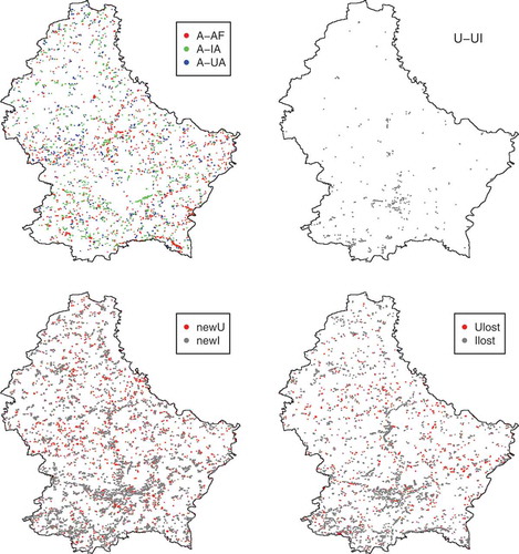
Figure 8. Architecture of the ML-CA-LTM model (drivers X1 − X16 are explained in Table 2; cell states are agriculture (1), forest (2), industrial (3) and urban (4)).

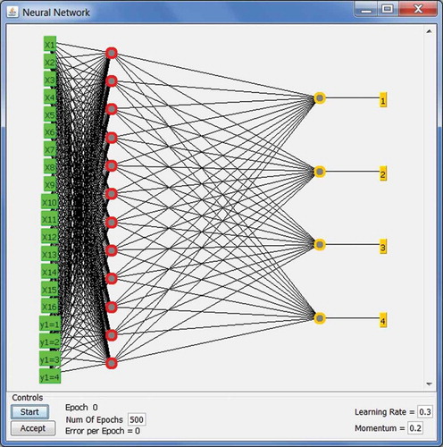
Table 4. Assessing the performance of the ML-CA-LTM model.

Accuracy	Precision	Recall	F1	Hamming loss
0.691 ± 0.021	0. 799 ± 0.009	0.728 ± 0.012	0.843 ± 0.006	0.131 ± 0.006

Figure 9. Observed versus predicted land use in 2007.

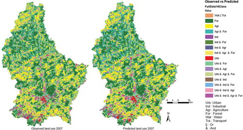
Figure 10. Map of hamming loss.

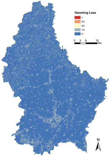
Figure 11. Confusion matrix with multi-labeling, observed versus predicted label set in 2007 (Note: normalized values between 0 and 100: each value in the original confusion matrix is divided by the sum of its corresponding line and multiplied by 100).

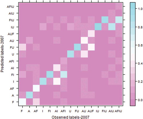
Table 5. Confusion matrix with mono-labeling, observed vs. predicted label set in 2007.

		Predicted label set in 2007
		U	I	A	F
Observed	U	741	69	354	100
	I	327	572	455	134
	A	132	87	296	436
	F	224	164	747	519

Table 6. Calculated accuracy metrics for ML-CA-LTM and ml-CA-LTM models (k = 3 and h = 12); based on 100 replications.

	ML-CA-LTM	ml-CA-LTM
Accuracy	0. 691 ± 0.021	0.397 ± 0.009
Precision	0. 799 ± 0.009	0.464 ± 0.009
Recall	0.728 ± 0.012	0.397 ± 0.009
F1	0.843 ± 0.006	0.414 ± 0.009
Accuracy [U]	0.885 ± 0.015	0.586 ± 0.009
Accuracy [I]	0.827 ± 0.016	0.384 ± 0.009
Accuracy [A]	0.917 ± 0.012	0.311 ± 0.009
Accuracy [F]	0.850 ± 0.011	0.314 ± 0.009
Precision [U]	0.578 ± 0.047	0.520 ± 0.009
Precision [I]	0.496 ± 0.053	0.641 ± 0.009
Precision [A]	0.935 ± 0.018	0.160 ± 0.009
Precision [F]	0.870 ± 0.020	0.437 ± 0.009
Recall [U]	0.710 ± 0.045	0.586 ± 0.009
Recall [I]	0.359 ± 0.083	0.384 ± 0.009
Recall [A]	0.961 ± 0.016	0.311 ± 0.009
Recall [F]	0.864 ± 0.019	0.314 ± 0.009
Build_time (seconds)	10.866 ± 0.106	5.69 ± 0.305

Zhang, M. L., and Z. H. Zhou. 2006. “Multilabel Neural Networks with Applications to Functional Genomics and Text Categorization.” IEEE Transactions on Knowledge and Data Engineering 18 (10): 1338–1351. doi:10.1109/TKDE.2006.162.

 Web of Science ®Google Scholar