Using low-density discrete Airborne Laser Scanning data to assess the potential carbon dioxide emission in case of a fire event in a Mediterranean pine forest

Figures & data

Figure 1. Land cover types of the study area and locations of 45 forest inventory plots.

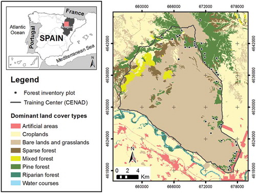
Table 1. Summary of the field plot data (n = 45).

Variable	Min	Max	Range	Mean	Standard deviation
Elevation (m)	246.7	722.5	475.9	467.9	156.7
Terrain slope (degrees)	0.7	25.7	25.0	10.7	7.3
Canopy cover (%)	16.1	93.0	76.8	62.9	19.2
Tree height (m)	3.7	11.3	7.6	7.1	2.0
dbh: breast height diameter (cm)	8.6	28.3	19.7	15.2	4.7
AGB: aboveground biomass (ton/ha)	1.0	112.1	111.1	37.5	27.9
Wr: belowground biomass (ton/ha)	0.4	32.7	32.3	13.2	7.4
TB: total biomass (ton/ha)	1.4	144.8	143.4	50.7	35.1

Figure 2. P. halepensis morphology and the tree biomass fractions according to Ruiz-Peinado, Del Rio, and Montero (2011). The total biomass (TB) refers to the dry weight of the plant material from trees, including roots, stems, bark, branches and leaves from the ground to the apex. The biomass of a tree can be divided into fractions above- and belowground (Maltamo, Næsset, and Vauhkonen 2014).

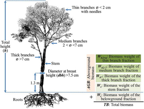
Table 2. Ranges applied to the variables influencing the accuracy of the estimations.

Variable	Source	Categories	Number of plots
Terrain slope (degrees)	ALS-derived DEM	Gentle (0–5)	11
		Moderate (5–15)	25
		Steep slopes (>15)	9
Aspect (degrees)	ALS-derived DEM	Indifferent (−1–0; 67.5–90; 247.5–270)	5
		Shady (0–67.5; 270–360)	19
		Sunny (90–247.5)	21
Canopy cover (%)	ALS data	Low (<40)	7
		Medium (40–70)	18
		High (>70)	20
Quantity of laser returns(number of points)	ALS data	Low (0–300)	9
		Medium (300–800)	21
		High (>800)	15
Scan angle (degrees)	ALS data	Low (0–±5)	23
		Medium (±5–±10)	10
		High (>±10)	12

Table 3. Correlation coefficients (Rho) describing the strength of linear relationships between plot-derived AGB and ALS-derived metrics.

Variable	Rho AGB	Variable	Rho AGB
Canopy height percentiles metrics (m)		Canopy height variability metrics (m)
P01	0.43**	Elev. standard deviation	0.72**
P05	0.67**	Elev. variance	0.72**
P10	0.85**	Elev. coefficient of variation	−0.36*
P20	0.94**	Elev. interquartile range	0.55**
P25	0.95**	Elev. skewness	−0.84**
P30	0.96**	Elev. kurtosis	0.50**
P40	0.96**	Canopy density metrics (%)
P50	0.96**	% First returns above 1 m	0.83**
P60	0.95**	% All returns above 1 m	0.64**
P70	0.95**	% First returns above mean height	0.88**
P75	0.95**	% First returns above mode height	0.38*
P80	0.95**	% All returns above mean height	0.78**
P90	0.94**	% All returns above mode height	0.15^ns
P95	0.91**	(All returns above 1 m)/(Total first returns) ∙ 100	0.84**
P99	0.89**
Canopy height metrics (m)		(All returns above mean)/(Total first returns) ∙ 100	0.88**
Elev. minimum	0.09^ns
Elev. maximum	0.89**	(All returns above mode)/(Total first returns) ∙ 100	0.38*
Elev. mean	0.96**
Elev. mode	0.93**

** and * denote significance (P-value < 0.01 and 0.05, respectively); ns denotes not significant (P-value > 0.05).

Figure 3. Metrics associated with the vertical distribution of ALS returns in three selected field plots representative of the P. halepensis forest: (a) smaller pines in open areas, (b) average height pines and (c) taller pines with little understory.

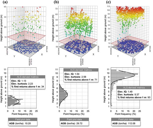
Table 4. Summary of stepwise selection.

Step	Variables entered	Partial R^2	Model R^2	Standard error of the estimate	F-value	Probability level > F
1	% First returns above 1 m	0.57	0.59	18.53	56.56	0.00
2	% First returns above 1 m Elev. interquartile range	0.50 0.24	0.66	16.36	42.85	0.00
3	% First returns above 1 m Elev. interquartile range Elev. kurtosis	0.36 0.55 0.55	0.84	11.15	77.98	0.00

Table 5. Model summary of AGB estimation.

Predictive model	Fitting phase				Cross-validation
	R^2	RMSE	%RMSE	Bias	R^2	RMSEcv	%RMSEcv	Bias
AGB = −61114.30 + 20201.17∙Elev. interquartile range +10,184.62∙Elev. kurtosis + 520.98% first returns above 1 m	0.84	10.65	27.39	0.00	0.84	10.63	27.35	0.03

Table 6. Kruskal–Wallis (K.W.) chi-square values for AGB.

Variable	K.W. chi-square	Asymptotic significance
Terrain slope	4.16	0.12
Aspect	1.40	0.50
Canopy cover	2.38	0.30
Quantity of laser returns	1.24	0.54
Scan angle	3.16	0.21

Statistical significance level at P-value <0.01.

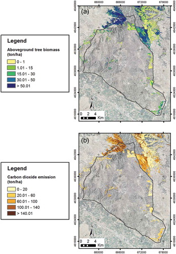
Figure 4. AGB (a) and CO₂ (b) emissions mapping of P. halepensis forest.

Ruiz-Peinado, R., M. Del Rio, and G. Montero. 2011. “New Models for Estimating the Carbon Sink Capacity of Spanish Softwood Species.” Forest Systems 20 (1): 176–188. doi:10.5424/fs/2011201-11643.

 Web of Science ®Google Scholar

Maltamo, M., E. Næsset, and J. Vauhkonen. 2014. Forestry Applications of Airborne Laser Scanning: Concepts and Case Studies. Managing Forest Ecosystems. London: Springer.

 Google Scholar