
Figures & data
Figure 1. Natural-color RapidEye scene of the study area in Germany. Brown indicates the dead trees (infested with bark beetles in 2011) extracted by the analysis of aerial photographs from 2012. White shading around brown areas indicates buffer zones of variable size around each infested area. The red box indicates a zoomed-in subset of the study area.
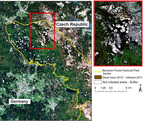
Figure 2. Overview of the data acquisition times in 2011. The green dots are the 8-day MODIS reflectance composites, purple dots are the RapidEye data used for training the data fusion, and red dots are the RapidEye data used as independent validation datasets.
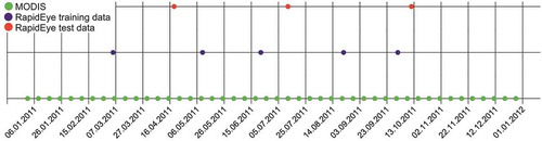
Figure 3. An example of variable buffers (purple) inserted around polygons of dead trees (green) of 2012. The linear relationship between the polygon and buffer sizes is shown in the upper-left corner.
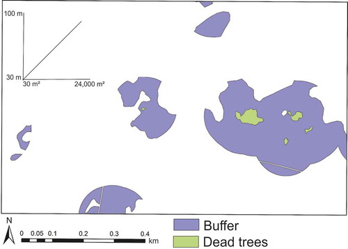
Figure 4. The workflow of FSDAF image fusion. The abbreviations t1 and t2 have been explained in Section 2.3.2.
Figure 5. Location of the pheromone traps overlapping a portion of the study site and the density of sampled beetles overlaid on a classification of synthetic RapidEye NDVI.
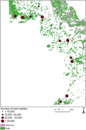
Figure 6. Scatterplots showing the correlation between the original independent validation and synthetic RapidEye data using the FSDAF method for 19 April (a), 12 July (b), and 22 November 2011. The 1:1 lines are dashed; the regression lines are solid. See text for values.
Figure 7. The NDVI range from 8-day composites of synthetic RapidEye data for 2011 overlaid on the locations of dead tree polygons (red) and buffered polygons (green) in 2012. On the missing dates, no cloud-free MODIS data were available. DOY refers to “day of year.”
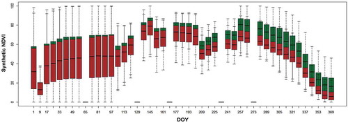
Figure 8. Results of conditional variable importance as mean decrease in accuracy of input image dates based on 100 repetitions of cforest.
Table 1. Accuracy assessment of the random forest classification of binary classes.
Figure 9. Examples of random forest maps of predicted classes and their classification probabilities. (a) Polygon-based classification, (b) wall-to-wall classification, (c) polygon-based classification probability of dead tree class, and (d) polygon-based classification probability of buffered zones. For clarity, all maps show only a subset of the entire study site.
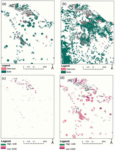
Table 2. Aggregated numbers of beetles counted per trap between 1 April and 30 September 2011 compared with the area classified as dead trees from synthetic RapidEye data in a buffer zone of 100 m radius around each trap.