Self-adaptive segmentation of satellite images based on a weighted aggregation approach

Figures & data

Figure 1. Study area images for (a) urban area, and (b) farmland area.

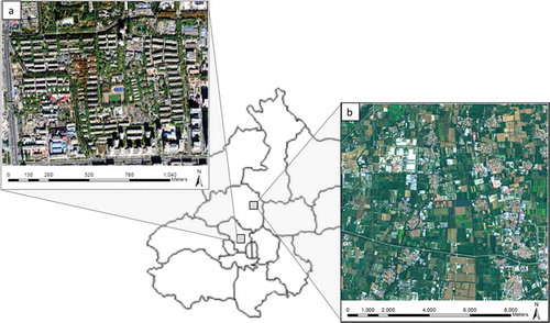
Figure 2. Flow chart for SAS, including three steps: (a) producing continuous multiscale segments by SWA approach; (b) calculating features for each scale from the first step and combining them later to learn selfhood scales; (c) finishing the merging based on the learned selfhood scales and generating self-adaptive results.

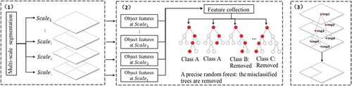
Figure 3. Flow chart for Segmentation by Weighted Aggregation (SWA) approach (Sharon et al. 2006).

Figure 4. Self-adaptive merging based on learned selfhood scales. (a) is the simplified tree representation of the workflow for self-adaptive merging. Each object in level 0 represented by leaf node searches for an appropriate segment bottom-up according to the learned selfhood scale, indicated by the corresponding color. Then the tree splits into subtrees with father nodes representing new segments. (b) is the concrete merging illustration. It shows the merging process of objects step by step.

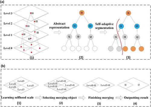
Figure 5. Multiscale results generated by SWA approach for urban area.

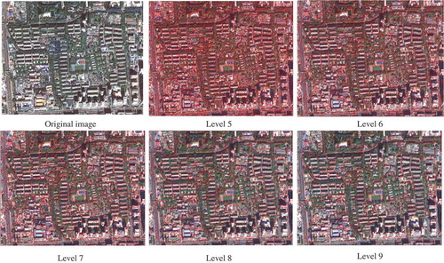
Figure 6. Multiscale results generated by SWA approach for farmland area.

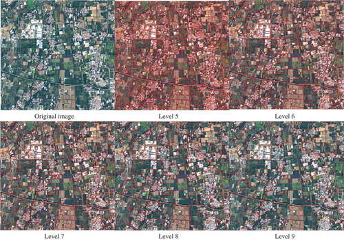
Figure 7. Selfhood scale learning results for (a) urban area and (b) farmland area. Each object was colored differently according to its selfhood scale learned from multiscale SWA results, ranging from level 5 to level 9.

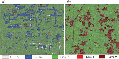
Table 1. The per-category proportions of different selfhood scales in urban area.

Proportion (%)	Level 5	Level 6	Level 7	Level 8	Level 9
Bright building	1.52	1.38	97.00	0.10	0
Dark building	6.48	19.44	74.07	0	0
Shadow	16.09	10.12	73.79	0	0
Road	0	0.35	99.65	0	0
Green vegetation	2.18	56.78	41.04	0	0
Red vegetation	4.09	9.21	65.98	0.51	20.20
Water	15.38	28.21	56.41	0	0
Total	6.53	17.93	72.56	0.09	2.89

The bold numbers represent the largest proportion for each category.

Table 2. The per-category proportions of different selfhood scales in farmland area.

Proportion (%)	Level 5	Level 6	Level 7	Level 8	Level 9
Bright building	0	0	98.59	0	1.41
Mixed residential area	0	0	8.23	0	91.77
Dark green farmland	0	0.88	98.83	0	0.29
Light green farmland	0	0	100.00	0	0
Bare soil	0	0	100.00	0	0
Road	0	0	11.11	0	88.89
Total	0	0.15	69.46	0	30.39

The bold numbers represent the largest proportion for each category.

Figure 8. A comparison between SWA and SAS results in urban area. (a) The original image and (b) the SAS result. A heterogeneous region, marked with yellow rectangle, is chosen to visually compare the six kinds of segmentation results at (c) level 5, (d) level 6, (e) level 7, (f) level 8, (g) level 9 of SWA results and (h) SAS result.

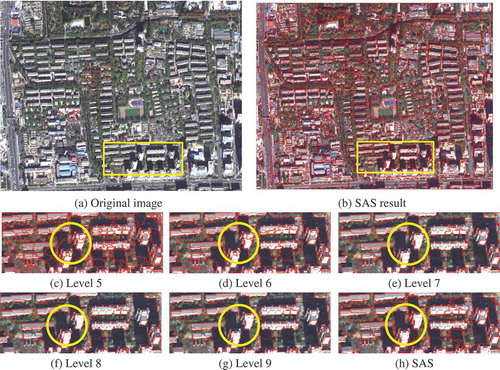
Figure 9. The manually delineated reference data used in geometry-based evaluation for (a) urban area and (b) farmland area.

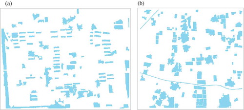
Figure 10. A comparison between SWA and SAS results in farmland area. (a) The original image and (b) the SAS result. A heterogeneous region, marked with yellow rectangle, is chosen to visually compare the six kinds of segmentation results at (c) level 5, (d) level 6, (e) level 7, (f) level 8, (g) level 9 of SWA results and (h) SAS result.

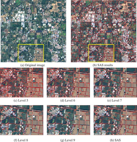
Table 3. Evaluation statistics of quantitative comparisons between SWA and SAS results (in urban area).

Methods	Scale	GS	OSeg	USeg	RMS
SWA	Level 5	0.463	0.731	0.010	0.518
	Level 6	0.410	0.467	0.065	0.370
	Level 7	0.330	0.227	0.160	0.267
	Level 8	0.373	0.183	0.445	0.430
	Level 9	0.433	0.184	0.607	0.540
SAS	-	0.328	0.296	0.044	0.236

The bold numbers represent the best segmentation results for each method.

Table 4. Evaluation statistics of quantitative comparisons between SWA and SAS results (in farmland area).

Methods	Scale	GS	OSeg	USeg	RMS
SWA	Level 5	0.308	0.794	0.010	0.562
	Level 6	0.268	0.545	0.029	0.401
	Level 7	0.227	0.237	0.086	0.218
	Level 8	0.233	0.101	0.365	0.326
	Level 9	0.251	0.025	0.637	0.466
SAS	-	0.202	0.147	0.096	0.167

The bold numbers represent the best segmentation results for each method.

Figure 11. A comparison between SWA and mean shift results in urban area.

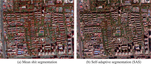
Table 5. Evaluation statistics of quantitative comparisons between mean shift and SAS results (in urban area).

Methods	GS	OSeg	USeg	RMS
Mean shift	0.452	0.304	0.163	0.389
SAS	0.328	0.296	0.044	0.236

Table 6. Evaluation statistics of quantitative comparisons between mean shift and SAS results (in farmland area).

Methods	GS	OSeg	USeg	RMS
Mean shift	0.447	0.325	0.124	0.342
SAS	0.202	0.147	0.096	0.167

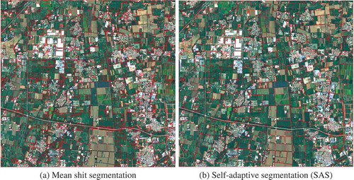
Figure 12. A comparison between SWA and mean shift results in farmland area.

Sharon, E., M. Galun, D. Sharon, R. Basri, and A. Brandt. 2006. “Hierarchy and Adaptivity in Segmenting Visual Scenes.” Nature 442: 810–813. doi:10.1038/nature04977.

 PubMed Web of Science ®Google Scholar