Figures & data
Table 1. Yearly publications of various data mining algorithms in the literature as indexed by Scopus and Web of Science. The title/abstract/keyword search was conducted on 18 October 2017, with the query ((“classification tree” or “regression tree” or “classification and regression tree” or CRT or “decision tree” or “random forest” or “neural net” or “neural network” or “support vector” or “k-means”) AND (“remote sensing” or “remotely sensed” or GIS or “geographic information science” or “satellite data” or “satellite imagery” or “satellite image”)). The query was filtered in each index to capture articles or articles in press published in the years 2013–2017. Duplicate records were removed. Some publications met the criteria of more than one data mining method.
Figure 1. Hypothetical classification or regression tree predicting parameter Z from the continuous variables W, Q, G, and X. The four ellipses are hierarchical splits based on a cost function that stratifies the data. Some example cost functions include minimizing the squared error, maximizing how pure the splits are – Gini index (Brownlee Citation2016), and high simplicity with a low absolute difference error – low sensitivity to outliers (Gu et al. Citation2016). The rectangles are the terminal node predictions. If Z is a categorical number, then the majority class is predicted (classification tree). If Z is a continuous value, the prediction can be the mean value or performed by either a simple regression or a multiple regression equation(s).
Figure 2. Optimization of the number of rules in a regression tree model to minimize overfitting tendencies and test error magnitudes. Score is (Test MAE – Training MAE) + test MAE and is a relative measure of model overfitting.
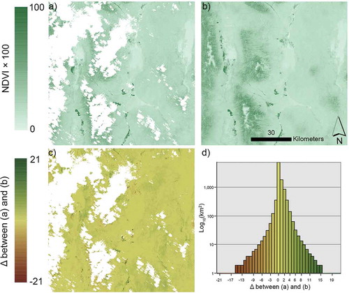
Figure 3. a) Normalized difference vegetation index (NDVI * 100) of Landsat 8 image acquired on 25 May 2016; b) NDVI synthetic Landsat image for 25 May 2106, generated with a regression tree model driven by Landsat OLI and Sentinel (MSI) time series data; c) Difference between real and synthetic images; and d) histogram of NDVI differences between real and synthetic images. Areas in white (no data) represent cloud, shadow, snow/ice, or water as identified from a decision tree masking model.