Incorporating the effect of ALS-derived DEM uncertainty for quantifying changes due to the landslide in 2011, Mt. Umyeon, Seoul

Figures & data

Figure 1. The location of the study area: (a) map of South Korea; (b) map of Seoul and the location of Mt. Umyeon; (c) aerial image of Mt. Umyeon in 2011.

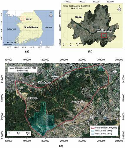
Table 1. Basic information about ALS data used in the study.

Category	Pre-event	Post-event
Acquisition date	15 August–16 September 2009 (exact date is unknown)	5 August 2011
Aircraft flying height	1500 m	1150 m
Flight speed	222.24 km/h	250 km/h
Laser scanner model	Leica ALS50-Ⅱ	Optech Gemini 167
Laser beam wavelength	73,500 Hz	70,000 Hz
Field of view	35°	44°
Point density	6	2.5
Coordinate system	Korea 2000/Central Belt 2010 (GRS80)

Figure 2. LiDAR data in the study area: (a) raw point cloud of 2009; (b) raw point cloud of 2011; (c) filtered points of 2009; (d) filtered points of 2011; (e) TIN model of 2009; (f) TIN model of 2011; (g) 1-m DEM of 2009; (f) 1-m DEM of 2011.

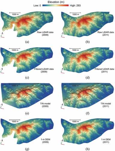
Figure 3. The spatial distribution of DoD in the study area.

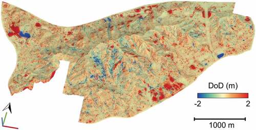
Figure 4. GNSS measurements in the study area: (a) the locations of the GNSS measurements overlayed on the point cloud; (b) boxplot of the elevation differences between GNSS measurements and LiDAR observations; (c) the elevation differences between GNSS measurements and LiDAR observations.

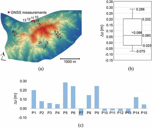
Figure 5. Vertical accuracy assessment by using stable terrain measurements: (a) location of road segments; (b) Box-and-whiskers plots representing the distribution of elevation differences of each road segment and the total.

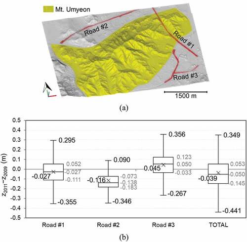
Figure 6. Spatial distribution of estimated error in the study area: (a) estimated error in the DEM of 2009; (b) estimated error in the DEM of 2011; (c) estimated error of DoD.

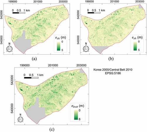
Figure 7. The probability calculated from DoD with uniformly distributed DEM error: (a) spatial distribution of t-score; (b) spatial distribution of the converted probability; (c) thresholded DoD with 68% confidence interval of the t-distribution; (d) thresholded DoD with 95% confidence interval of the t-distribution.

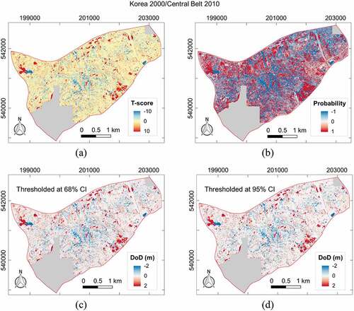
Figure 8. The probability updated by Bayes Theorem with uniformly distributed uncertainty: (a) the probability revealed from spatial index analysis; (b) the conditional posterior probability; (c) thresholded DoD with 68% confidence interval; (d) thresholded DoD with 95% confidence interval.

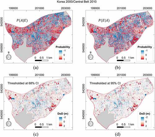
Figure 9. The probability calculated from DoD with spatially distributed DEM error: (a) spatial distribution of t-score; (b) spatial distribution of the converted probability; (c) thresholded DoD with 68% confidence interval of the t-distribution; (d) thresholded DoD with 95% confidence interval of the t-distribution.

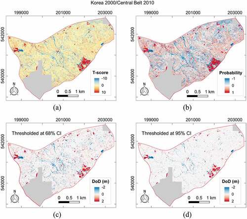
Figure 10. The probability updated by Bayes Theorem with spatially distributed uncertainty: (a) the probability revealed from spatial index analysis; (b) the conditional posterior probability; (c) thresholded DoD with 68% confidence interval; (d) thresholded DoD with 95% confidence interval.

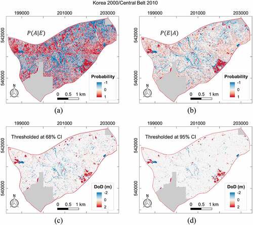
Table 2. Volumetric changes over whole study area.

Volumetric DoD	Erosion	Deposition	Net
Unthresholded (no uncertainty)	2,214,562	3,119,195	904,633
Standard minLoD	2,087,369	2,992,826	905,457
Uniform DEM uncertainty (95% CI)	1,828,396	2,692,010	863,614
Spatially distributed DEM uncertainty (95% CI)	802,051	1,045,214	243,163
Bayesian updating with uniform DEM uncertainty (95% CI)	1,318,280	2,092,445	774,165
Bayesian updating with spatially distributed DEM uncertainty (95% CI)	705,807	933,901	228,093

(Unit: ${\mathrm{m}}^3$).

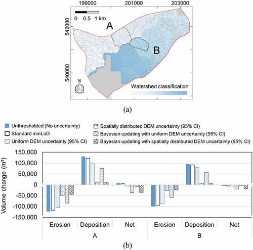
Table 3. Volumetric changes of small-scale watershed areas, A and B.

Volumetric DoD	A			B
	Erosion	Deposition	Net	Erosion	Deposition	Net
Unthresholded (no uncertainty)	123,266	130,443	7,177	100,020	95,520	−4,500
Standard minLoD	117,896	122,490	4,593	96,763	91,826	−4,937
Uniform DEM uncertainty (95% CI)	105,856	99,684	−6,172	86,648	80,444	−6,204
Spatially distributed DEM uncertainty (95% CI)	49,779	12,979	−36,800	26,634	7,450	−19,184
Bayesian updating with uniform DEM uncertainty (95% CI)	84,548	75,179	−9,369	59,328	56,202	−3,126
Bayesian updating with spatially distributed DEM uncertainty (95% CI)	45,832	10,100	−35,731	23,553	5,305	−18,248

(Unit: ${\mathrm{m}}^3$).

Figure 11. Volumetric changes in small-scale areas, A and B: (a) The location of selected areas; (b) Graph with different thresholding criteria.