Spatiotemporal mixed effects modeling for the estimation of PM_2.5 from MODIS AOD over the Indian subcontinent

Figures & data

Figure 1. Measured PM_2.5 concentrations (μg/m³) across 33 ground monitoring stations for the study area during January 2017 – August 2017. Tamil Nadu and Punjab states shaded in gray color are chosen for the study on Gap filling where AOD values are missing (Section 4.2 and 5.2).

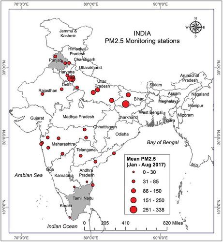
Figure 2. Methodology adopted for the estimation of daily PM_2.5 from MODIS AOD over the Indian subcontinent.

Figure 3. Proportionate extent of (a) Agricultural area (b) Road density (c) Forest cover (d) Open spaces calculated within 10 km × 10 km grid.

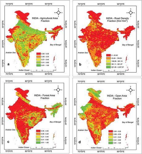
Figure 4. Percentage availability of AOD data during the study period of January – August 2017 for the Indian sub-continent.

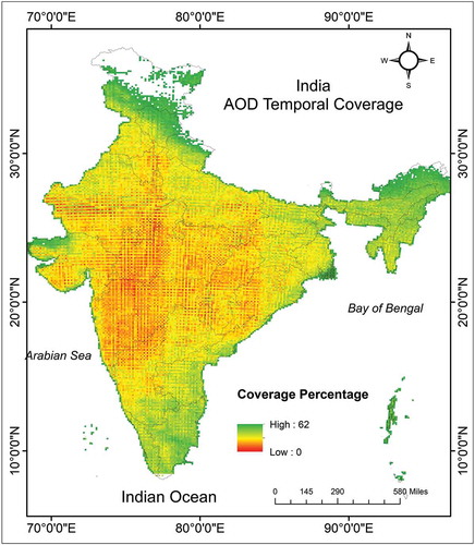
Table 1. Statistical summary of parameters associated with the spatiotemporal mixed effects model.

Parameters	STMEM	LMEM
Number of Stations (i)	33	33
Number of Days (j)	157	168
Number of co-incident observations of AOD and PM2.5 (Temperature observations included for STMEM)	599	885
Number of Fixed Effect Coefficients	7	2
Number of Random Effect Coefficients	661	369

Figure 5. Scatterplot showing the measured and estimated PM_2.5 (μgm/m³) using spatiotemporally modified MEM with the combination of variables (a) M1 – Open spaces and Agricultural area (OA with cross); (b) M2 – Open spaces and Forest cover (OF with minus); (c) M3 – Open spaces, Agricultural area, Forest cover area and Temperature data (OAFT with plus); (d) M4 – Open spaces, Agricultural area, Forest cover area, Temperature and Road density data (OAFTR with dots).

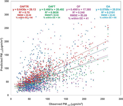
Figure 6. Validation of LMEM and STMEM outputs against observed PM_2.5 levels across 33 stations between January and August 2017.

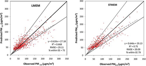
Table 2. Values of fixed effect coefficients of the spatiotemporal mixed effects model including road density $(\gamma$₁₎, open spaces ($\gamma$₂), agricultural area ($\gamma$₃), and forest cover ($\gamma$₄).

Variables		STMEM	LMEM
Fixed Intercept α		3.977	4.417
Fixed Slope (AOD) β1		1.627 * 10^−4	2.050 * 10^−4
Fixed Slope (Temp) β2		−1.830 * 10^−2	-
Fixed coefficients	Road density ($\gamma$1)	1.156	-
	Open space ($\gamma$2)	0.692	-
	Agriculture ($\gamma$3)	0.817	-
	Forest Cover ($\gamma$4)	4.800 * 10^−4	-
Mean Random Intercept (uj)		5.312 * 10^−6	0.169
Mean Random AOD Slope (vj)		6.769 * 10^−5	2.3965 * 10^−4
Mean Site Bias (si)		1.7 * 10^−4	0.391
Mean Random Temperature Slope (kj)		−0.005	-

Figure 7. Estimated PM_2.5 concentrations (μg/m³) during January – August 2017 (a – h), Minimum (i) and Maximum (j) for Indian subcontinent using spatiotemporal mixed effects model including open spaces, forest cover, agricultural areas, road density, and temperature.

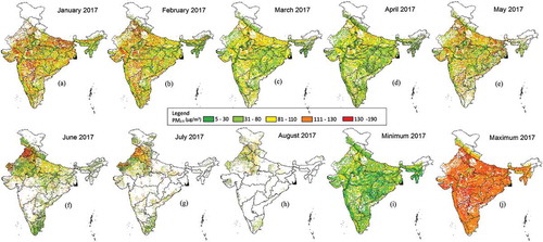
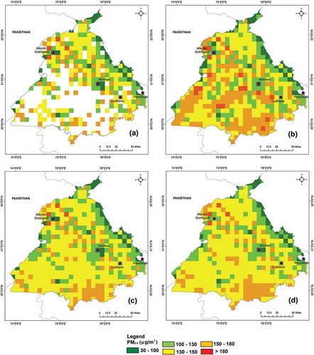
Figure 8. (a) PM_2.5 concentrations for April 2017 (b) Gap – filled spatiotemporal interpolation by mixed effects model implemented using spline interpolation (c) using ordinary kriging (d) using the IDW method of Tamil Nadu.

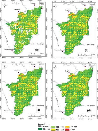
Figure 9. (a) PM_2.5 concentrations for April 2017 (b) Gap – filled spatiotemporal interpolation by mixed effects model implemented using spline interpolation (c) using Ordinary Kriging (d) using the IDW method for Punjab.