Comparative performance of convolutional neural network, weighted and conventional support vector machine and random forest for classifying tree species using hyperspectral and photogrammetric data

Figures & data

Figure 1. Study areas and samples location. (a) Santa Catarina state; (b) Curitibanos municipality; (c) Zoom showing the areas location (Google Earth); (d) Area 1; (e) Area 2.

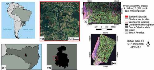
Table 1. Characteristics of the camera, flight and data acquired in the study areas.

Characteristic	Description
Focal length	8.6 mm
Field of view	37°
Spatial resolution	11 cm (Area 1) 12 cm (Area 2)
Image dimensions	1,023 × 648 pixels
Flight height/speed	150 m/4m.s
Number of strips	8 (Area 1) 6 (Area 2)
Forward and side overlap	70 and 60% (Area 1) 60 and 50% (Area 2)
PPC density	35 points.m^−2 (Area 1) 25 points.m^−2 (Area 2)

Table 2. Tree species and their respective successional groups and number of ITCs and pixels for each tree species used in the classification process according to the study area (A1 = Area 1 and A2 = Area 2).

				ITCs		Pixel samples
ID	Species	Family	Successional group	A1	A2	A1	A2
a	Luehea divaricata	Malvaceae	initial or late secondary, climatic	5	4	23,624	15,259
b	Araucaria angustifolia	Araucariacea	pioneer or secondary	8	6	27,191	32,925
c	Mimosa scabrella	Fabaceae	pioneer	7	-	25,449	-
d	Lithraea brasiliensis	Anacardiaceae	pioneer, initial secondary or climatic	5	8	17,458	13,553
e	Campomanesia xanthocarpa	Myrtaceae	initial or late secondary	5	3	18,837	7,565
f	Cedrela fissilis	Meliaceae	initial or late secondary, climatic	5	2	24,368	12,910
g	Cinnamodendron dinisii	Canellaceae	late secondary	5	-	6,927	-
h	Cupania vernalis	Sapindaceae	initial or late secondary	5	-	12,475	-
i	Matayba elaeagnoides	Sapindaceae	late secondary	8	-	48,231	-
j	Nectandra megapotamica	Lauraceae	initial or late secondary	8	4	11,247	4,862
k	Ocotea sp.	Lauraceae	initial secondary	9	3	101,884	12,991
l	Podocarpus lambertii	Podocarpaceae	late secondary or climatic	6	4	12,387	21,391
m	Schinus terebethifolius (sp1)	Anacardiaceae	pioneer, initial or late secondary	2	2	4,491	2,646
n	Schinus lentiscifolius (sp2)	Anacardiaceae	initial or late secondary	2	-	6,083	-
o	Erythrina falcata	Fabaceae	initial secondary or climatic	-	2	-	3,663
p	Sebastiania commersoniana	Euphorbiaceae	initial secondary	-	3	-	3,396

Table 3. Description of features used in this study.

Group	Feature name	Description	Equation	Reference
Spectral bands	VNIR	Wavelengths (ρ) 506 to 819 nm
MNF	MNF	Minimum noise fraction		Green et al. (1988)
VIs	NDVI	Normalized Difference Vegetation Index	NDVI = $\frac{{\rho }_{750}-{\rho }_{650}}{{\rho }_{750}+{\rho }_{650}}$	Rouse et al. (1973)
	PRI	Photochemical reflectance index	PRI = $\frac{{\rho }_{535}-{\rho }_{565}}{{\rho }_{535}+{\rho }_{565}}$	Gamon, Peñuelas, and Field (1992)
	PSRI	Plant senescence reflectance index	PSRI = $\frac{{\rho }_{679}-{\rho }_{506}}{{\rho }_{750}}$	Merzlyak et al. (1999)
	PSSR	Pigment specific simple ratio	PSSR = $\frac{{\rho }_{819}}{{\rho }_{679}}$	Blackburn (1998)
GLCM	SM	Angular second moment	SM = ${\sum }_{i,j=0}^{N-1}\left\{p{\left(i,j\right)}^2\right\}$	Haralick, Shanmugam, and Dinstein (1973)
	con	Contrast	Con = ${\sum }_{i,j-0}^{N-1}pi,j{\left(i-j\right)}^2$
	var	Variance	Var =${\sum }_{i,j=0}^{N-1}{\left(i-\mu \right)}^{2}p\left(i,j\right)$
	hom	Homogeneity	Hom = ${\sum }_{i,j=0}^N\frac{pi,j}{1+{\left(1-j\right)}^2}$
	cor	Correlation	Cor =${\sum }_{i,j=0}^{N}pi.j\frac{\left[\left(i-\mu i\right)\left(j-\mu j\right)\right]}{\sqrt{\left({\sigma }^{2}i\right)\left({\sigma }^{2}j\right)}}$
	ent	Entropy	Ent =
	dis	Dissimilarity	Dis = ${\sum }_{i,j-0}^{N-1}pi,j\left|1-j\right|$
	mean	Textural mean	Mean = $\frac{{\sum }_{i=1}^{N}pxi}{N}$
CHM	CHM	Canopy height model	CHM = $DSM-DTMLiDAR$
PPC	zmax	maximum height of all the points within each pixel
	zmean	mean of all the height points within each pixel
	zq90	90th percentile of height distribution within each pixel
	zq70	70th percentile of height distribution within each pixel
	zq5	5th percentile of height distribution within each pixel
	zentropy	entropy of height distribution within each pixel

Table 4. Description of the datasets according to the features used in the classification process.

Dataset Name	VNIR	CHM	PPC	MNF	GLCM	VI	Total features
VNIR	25	-	-	-	-	-	25
VNIR_CHM	25	1	-	-	-	-	26
VNIR_PPC^a	25	-	6	-	-	-	31
VNIR_PPC_CHM	25	1	6	-	-	-	32
VNIR_PPC_CHM_MNF^a	25	1	6	8	-	-	40
VNIR_PPC_CHM_GLCM^a	25	1	6	-	24	-	56
VNIR_PPC_CHM_VI^a	25	1	6	-	-	4	36
VNIR_PPC_CHM_MNF_VI^a	25	1	6	8	-	4	44
VNIR_MNF_GLCM_VI^a	25	-	-	8	24	4	61
MNF_PPC_CHM^a	-	1	6	8	-	-	15
MNF_PPC_CHM_VI^a	-	1	6	8	-	4	19
FSJM-A1^a	18	1	6	7	10	4	46
FSJM-A2^a	21	1	6	4	14	3	49
full^a	25	1	6	8	24	4	68

^aDatasets not tested in the wSVM and CNN algorithms.

Figure 2. Average accuracy of the 5-fold cross validation procedure to find the best SVM parameters for each dataset. Note: This figure shows the best (right) and worst (left) dataset result for Area 1.

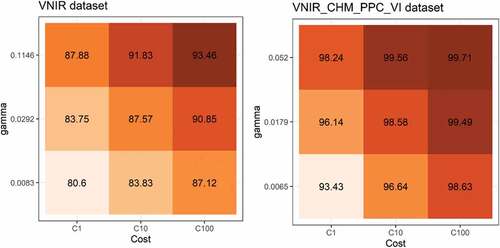
Figure 3. CNN architecture for Area 1 with 25 bands and 15 classes (14 tree species plus “background” class).

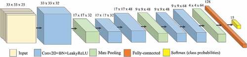
Figure 4. Variable importance according to the JM distance for each study area. The features are described in .Table 3

Figure 5. Mean radiance (with standard deviation) of the tree species classified in Area 1 (a) and Area 2 (b).

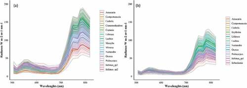
Figure 6. Boxplots showing the distribution of the PPC (zmax and zq5) and CHM values of the tree species samples in Area 1 (a and b) and Area 2 (c and d). The central lines within each box are the medians. The boxes edges represent the upper and lower quartiles. Outliers are plotted individually.

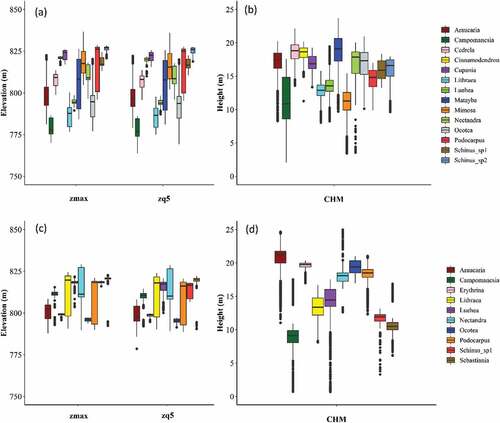
Table 5. Classification results according to the area/classifier/dataset/approach. The best result for each classifier/approach is highlighted.

		Area 1		Area 2
Classifier	Dataset	OA (%)	Kappa	OA (%)	Kappa
SVM	VNIR	62.67	0.57	48.91	0.41
	VNIR_CHM	67.90	0.63	63.93	0.58
	VNIR_PPC	68.61	0.64	51.50	0.44
	VNIR_CHM_PPC	76.04	0.73	63.10	0.57
	VNIR_CHM_PPC_MNF	76.55	0.73	62.35	0.57
	VNIR_CHM_PPC_GLCM	74.56	0.71	61.98	0.56
	VNIR_CHM_PPC_VI	77.66	0.74	62.94	0.57
	VNIR_CHM_PPC_MNF_VI	77.10	0.74	62.25	0.56
	VNIR_MNF_GLCM_VI	61.91	0.56	47.34	0.39
	MNF_CHM_PPC	68.97	0.64	56.47	0.50
	MNF_CHM_PPC_VI	73.60	0.70	59.06	0.53
	FSJM	74.68	0.71	57.66	0.52
	full	72.59	0.68	61.90	0.56
	MV best SVM result for each area*	82.52	0.80^1	75.47	0.72^1
	OBIA (VNIR_CHM_PPC_VI)	73.52	0.69	-	-
RF	VNIR	59.24	0.52	48.60	0.40
	VNIR_CHM	66.06	0.60	66.02	0.61
	VNIR_PPC	51.46	0.44	63.43	0.58
	VNIR_CHM_PPC	55.91	0.50	65.45	0.60
	VNIR_CHM_PPC_MNF	57.54	0.52	65.94	0.60
	VNIR_CHM_PPC_GLCM	56.60	0.50	66.51	0.61
	VNIR_CHM_PPC_VI	55.59	0.49	65.61	0.60
	VNIR_CHM_PPC_MNF_VI	56.71	0.51	66.21	0.61
	VNIR_MNF_GLCM_VI	59.17	0.52	48.97	0.40
	MNF_CHM_PPC	52.72	0.46	61.72	0.56
	MNF_CHM_PPC_VI	53.82	0.47	63.28	0.57
	FSJM	56.32	0.50	52.08	0.46
	full	57.74	0.52	67.37	0.62
	OBIA(VNIR_CHM_PPC_VI_MNF)	68.00	0.63	-	-
wSVM	VNIR	56.42	0.51	48.98	0.42
	VNIR_CHM_PPC	74.37	0.71	65.15	0.60
	best SVM result for each area*	75.03	0.72	65.60	0.60
CNN	VNIR	84.37	0.82^1	74.95	0.71^1
	VNIR_CHM_PPC	77.17	0.74	70.36	0.65
	VNIR_CHM	79.19	0.76	73.12	0.69^1

*Majority vote (MV) procedure and the wSVM classifier applied to the VNIR_CHM_PPC_VI dataset in Area 1 and the VNIR_CHM dataset in Area 2. ¹Best results that do not significantly differ among themselves according to the z test.

Figure 7. Differences in overall accuracy with the inclusion of features and approaches in relation to the VNIR dataset, using the SVM and RF classifiers.

Figure 8. F-measures of each tree species class for Area 1 according to the classifier. Black bars indicate the minimum and maximum values varying according to the employed dataset.

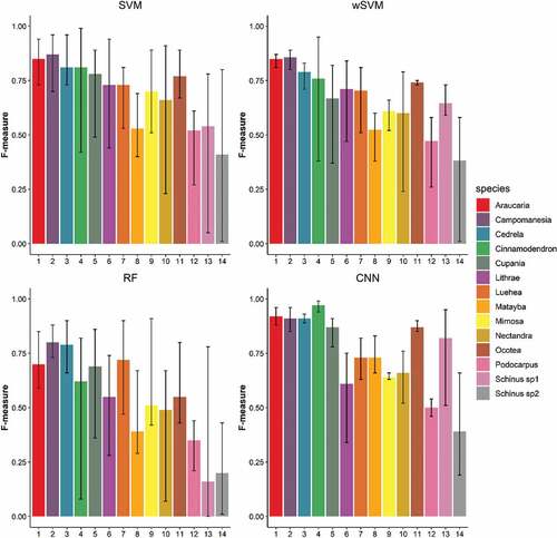
Figure 9. F-measures of each tree species class for Area 2 according to the classifier. Black bars indicate the minimum and maximum values varying according to the dataset.

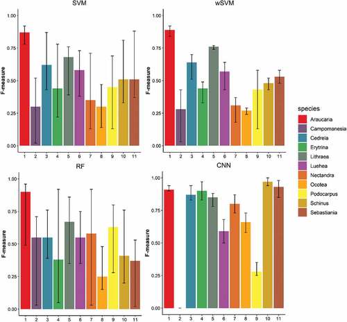
Figure 10. Some of the confusion matrices of Area 1 (top) and Area 2 (bottom). Note: Classes identified according to the species ID presented in .Table 2

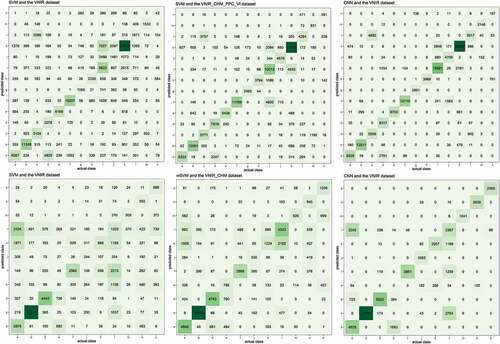
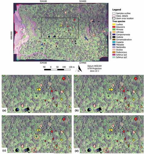
Figure 11. Examples of classification images for Area 1. a) Reference samples; b) the SVM classifier (VNIR_CHM_PPC dataset) after the MV rule – the red circle shows missing ITCs of Podocarpus; c) OBIA associated with the RF classifier and the VNIR_CHM_PPC_VI_MNF dataset – the red circle shows two missing ITCs of Nectandra and one of Podocarpus; d) the CNN classifier with the VNIR dataset – the red circle shows one missing ITC of Nectandra.

Green, A. A., M. Berman, P. Switzer, and M. D. Craig. 1988. “A Transformation for Ordering Multispectral Data in Terms of Image Quality with Implications for Noise Removal.” IEEE Transactions on Geoscience and Remote Sensing 26: 65–74. doi:10.1109/36.3001.

 Web of Science ®Google Scholar

Rouse, J. W., R. H. Haas, J. A. Schell, and W. D. Deering. 1973. “Monitoring Vegetation Systems in the Great Plains with ERTS.” Paper presented at Third ERTS Symposium, NASA SP-351, Washington, December 14, 309–317.

 Google Scholar

Gamon, J. A., J. Peñuelas, and C. B. Field. 1992. “A Narrow-waveband Spectral Index that Tracks Diurnal Changes in Photosynthetic Efficiency.” Remote Sensing of Environment 41: 35–44. doi:10.1016/0034-4257(92)90059-S.

 Web of Science ®Google Scholar

Merzlyak, M. N., A. A. Gitelson, O. B. Chivkunova, and V. Y. Rakitin. 1999. “Non Destructive Optical Detection of Pigment Changes during Leaf Senescence and Fruit Ripening.” Physiologia Plantarum 106 (1): 135–141. doi:10.1034/j.1399-3054.1999.106119.x.

 Web of Science ®Google Scholar

Blackburn, G. A. 1998. “Spectral Indices for Estimating Photosynthetic Pigment Concentrations: A Test Using Senescent Tree Leaves.” The International Journal of Remote Sensing 19 (4): 657–675. doi:10.1080/014311698215919.

 Web of Science ®Google Scholar

Haralick, R. M., K. Shanmugam, and I. H. Dinstein. 1973. “Textural Features for Image Classification.” IEEE Transactions on Systems, Man, and Cybernetics 3: 610–621. doi:10.1109/TSMC.1973.4309314.

 Web of Science ®Google Scholar