The impact of voxel size, forest type, and understory cover on visibility estimation in forests using terrestrial laser scanning

Figures & data

Table 1. The basic information of the 24 forest plots. The three coverage levels of understory vegetation are low (<18%), medium (18–34%), and high (>34%)

Plot ID	Elevation (m)	Slope (°)	Understory cover (%)	Understory cover level	Forest type
1	935	9.39	2	low	deciduous
2	842	9.13	7	low	deciduous
3	862	8.54	17	low	deciduous
4	843	6.56	21	medium	deciduous
5	930	8.33	23	medium	deciduous
6	932	6.10	34	medium	deciduous
7	1076	7.35	46	high	deciduous
8	766	1.60	47	high	deciduous
9	866	9.63	3	low	coniferous
10	777	0.87	8	low	coniferous
11	853	7.67	11	low	coniferous
12	752	3.13	18	medium	coniferous
13	802	9.02	25	medium	coniferous
14	779	9.98	28	medium	coniferous
15	740	3.68	35	high	coniferous
16	1045	6.38	45	high	coniferous
17	788	5.83	5	low	mixed
18	800	3.58	10	low	mixed
19	764	6.64	19	medium	mixed
20	771	6.59	23	medium	mixed
21	829	8.19	35	high	mixed
22	828	5.21	39	high	mixed
23	803	7.25	42	high	mixed
24	857	8.46	44	high	mixed

Figure 1. The location and distribution of sampling plots in the Bavarian Forest National Park, Germany

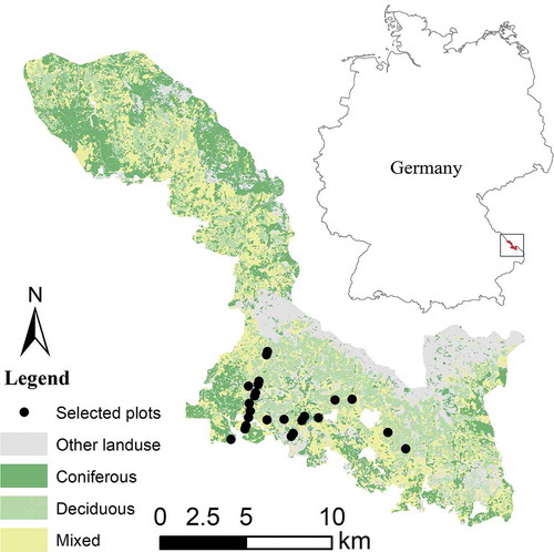
Figure 2. (a) A schematic of the sample plot design with a radius of 20 m, (b) the setup with cover board, reflector, and camera

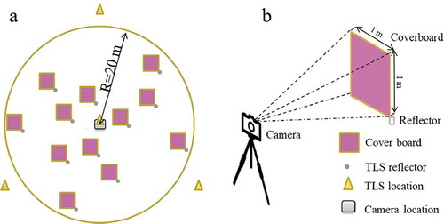
Table 2. The spectral variables used in the stepwise logistic regression to classify board versus non-board on the cover board photos

Variable	Abbreviation	Calculation
Red	R	8-bit R pixel mean
Green	G	8-bit G pixel mean
Blue	B	8-bit B pixel mean
Normalized red	$R_{norm}$	R/(R + G + B)
Normalized green	$G_{norm}$	G/(R + G + B)
Normalized blue	$B_{norm}$	B/(R + G + B)
Magenta	M	(R + B)/2
Cyan	C	(B + G)/2
Yellow	Y	(G + R)/2
Normalized magenta	$M_{norm}$	M/(M + C + Y)
Normalized cyan	$C_{norm}$	C/(M + C + Y)
Normalized yellow	$Y_{norm}$	Y/(M + C + Y)
Normalized difference red-green	NDRG	(R – G)/(R + G)
Normalized difference green-blue	NDGB	(G – B)/(G + B)
Normalized difference blue-red	NDBR	(B – R)/(B + R)
Normalized difference magenta-cyan	NDMC	(M – C)/(M + C)
Normalized difference cyan-yellow	NDYC	(C – Y)/(C + Y)
Normalized difference yellow-magenta	NDYM	(Y – M)/(Y + M)

Figure 3. Illustration of occupancy grid mapping: (a) A 2D example of mapping the occupancy probabilities of the cells affected by one laser beam. The orange arrow represents a laser beam. $d_n$ is the distance from the point $m_n$ to the TLS sensor origin. $s_i$ is the i-th voxel which lies on the traveling path of the laser beam that raised the point $m_n$. Lower probabilities are encoded in white, higher probabilities in black. The unmapped cells are gray. (b) Inverse sensor model for one laser beam. Occupancy probability values for the distance measure at 5 m. (c) A 2D example of mapping the occupancy probabilities of two cells affected by several laser beams. One cell at 6 m from the TLS sensor contains five points, and another one at 10 m from the TLS sensor contains three points. The brown and green solid lines and dots represent laser beams and points, respectively. (d) The resulting occupancy probability values for the two cells in (c)

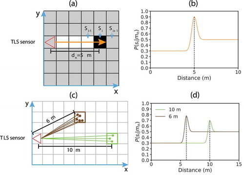
Table 3. The standard occupancy grid mapping algorithm, shown here using log-odds representations

/* Initialization */ for all grid voxels (x, y, z) dolx,y,z = log p(sx,y,z) –log[1–p (sx,y,z)]endfor /* Grid update using log-odds */ for all points t from 1 to n do for all grid cells (x, y, z) in the perceptual range of do lx,y,z = lx,y,z +log p(sx,y,z Vmt) –log[1–p(sx,y,z) Vmt] +log[1–p(sx,y,z)] endfor endfor /* Recovery of occupancy probabilities */ for all grid cells (x, y, z) doendfor

Figure 4. Illustration of the voxelization of a sample point cloud (Plot 12) using five different voxel sizes

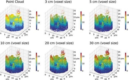
Table 4. The confusion matrix for the classification results of cover board photos

		Reference		Accuracy
		Board	Non-board	User	Producer	Overall
Prediction	Board	94	4	96%	94%	95%
	Non-board	6	96	94%	96%

Figure 5. An example of the classification results of the cover board photos. The left, middle, and right panels correspond to the mixed, coniferous, and deciduous forest plots, respectively. In binary images, black areas indicate pixels classified as a board and white areas indicate pixels classified as a non-board

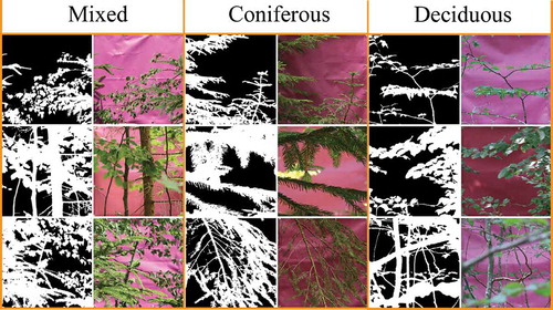
Table 5. Summary of results from a factorial ANOVA showing the effects of forest type, understory cover, voxel size, and their interaction on the agreement between photography-derived and TLS-derived visibility

Response variables	Factors	SS	d.f.	MS	F-value	p-value	Partial ${\eta }^2$
$R^2$	Forest type	0.427	2	0.2137	46.65	0.000*	0.41
	Understory cover	0.362	2	0.1812	39.53	0.000*	0.37
	Voxel size	6.950	4	1.7375	379.22	0.000*	0.92
	Forest type × Understory cover	0.297	4	0.0742	16.20	0.000*	0.32
	Forest type × Voxel size	0.035	8	0.0044	0.96	0.469	0.05
	Understory cover × Voxel size	0.076	8	0.0095	2.08	0.042*	0.11
	Forest type × Understory cover × Voxel size	0.102	16	0.0063	1.39	0.158	0.14
	Residuals	0.619	135	0.0046	-	-	-
RMSE	Forest type	274.7	2	137.3	16.19	0.000*	0.19
	Understory cover	589.9	2	295.0	34.77	0.000*	0.34
	Voxel size	2872.9	4	718.2	84.67	0.000*	0.72
	Forest type × Understory cover	322.1	4	80.5	9.50	0.000*	0.22
	Forest type × Voxel size	99.7	8	12.5	1.47	0.174	0.08
	Understory cover × Voxel size	59.3	8	7.4	0.86	0.540	0.05
	Forest type × Understory cover × Voxel size	161.1	16	10.1	1.19	0.286	0.12
	Residuals	1145.2	135	8.5	-	-

SS = sum of squares, d.f. = degrees of freedom, MS = mean square, * p < 0.05.

Figure 6. The mean of $R^2$ and RMSE between photography-derived and TLS-derived visibility (a) for five different voxel sizes: 3 cm, 5 cm, 10 cm, 20 cm, 30 cm, (b) for three forest types: deciduous, coniferous, and mixed, and (c) three levels of understory cover: low, medium, and high. The different letters inside the figures indicate a statistically significant difference between different combinations of these three factors. The same letter indicates no significant difference (Tukey’s HSD test, p < 0.05)

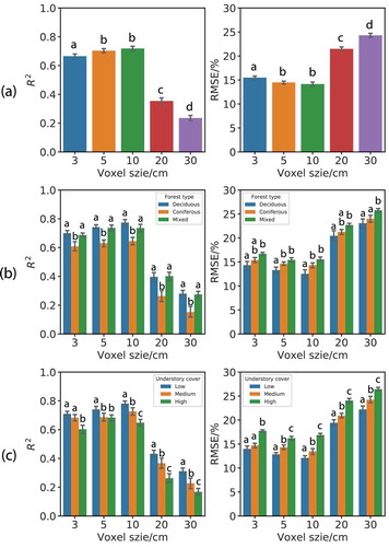
Table 6. The agreement ($R^2$ and RMSE) between photography-derived and TLS-derived visibility under different forest types and understory cover conditions using a voxel size of 10 cm

	Forest type			Understory cover			overall
	Deciduous	Coniferous	Mixed	Low	Medium	High
$R^2$	0.79	0.73	0.73	0.77	0.72	0.67	0.77
RMSE (%)	12.45	14.34	16.07	13.37	13.74	17.29	14.33

Figure 7. (a) The relationship between the average ratio of unmapped voxels of all 24 plots and voxel size, (b) the average ratio of unmapped voxels of all 24 plots for different levels of understory cover given a voxel size of 10 cm

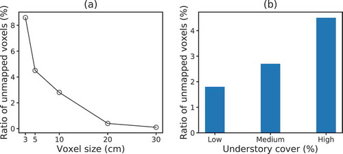
Table 7. Summary of results from a one-way ANOVA showing the effect of the traveling distance of the laser beam on the agreement between photography-derived and TLS-derived visibility

Response variables	Factors	SS	d.f.	MS	F-value	p-value
$R^2$	Distance	0.010	3	0.0034	0.549	0.654
	Residuals	0.125	20	0.0063	-	-
RMSE	Distance	18.05	3	6.017	1.191	0.338
	Residuals	101.02	20	5.051	-

SS = sum of squares, d.f. = degrees of freedom, MS = mean square, p < 0.05.