Figures & data
Figure 1. Color composite of a Landsat 8 image over the SMAPVEX16-MB field campaign area (Colliander et al. Citation2019). In total, 9 RISMA stations and 50 temporary agricultural fields are shown by green stars and red rectangles, respectively. The inset shows the arrangements of the 16 sample sites within two different fields
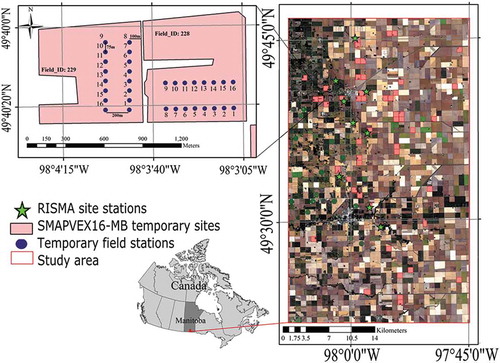
Figure 2. SRTM global digital elevation map and location of the centers of the dense in situ validation sites. The selected sites are shown by red circles. Also, those sites that do not meet the time interval, station number, and geographic distribution criteria are illustrated by green, blue, and black circles, respectively
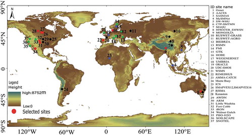
Figure 3. Schematic diagram of the methodology emphasizing three steps of the proposed method
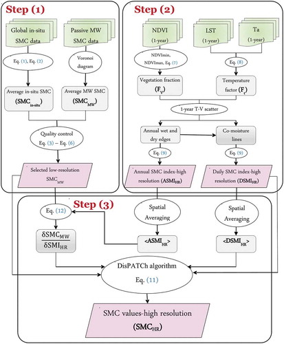
Figure 4. The Kenaston field campaign. Those stations distributed in an area equal to the standard MW product grid size (filled blue rectangle) are selected for the validation process. Lines show the SMAP global grid area
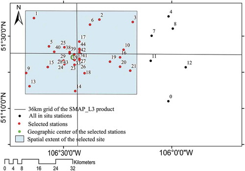
Figure 5. A typical 1-year T-V scatter plot with its annual wet and dry edges and some imaginary co-moisture lines between them. A hypothetical 1-day scatter plot and the daily wet and dry edges are also shown in this figure
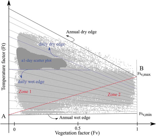
Table 1. SMMW validation sites with the number by which they are shown in
Figure 6. Scatter plots of daily soil moisture estimates from field stations versus AMSR2, SMOS, and SMAP soil moisture products at eight validation sites
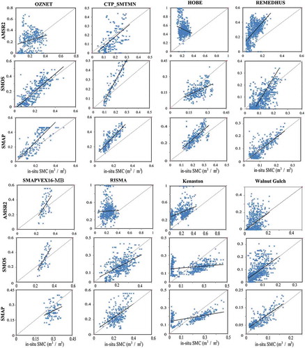
Table 2. Summarized resultant statistical indicators for the AMSR2, SMOS, and SMAP products
Figure 7. Percentage of cases where SMAP or SMOS products rank best
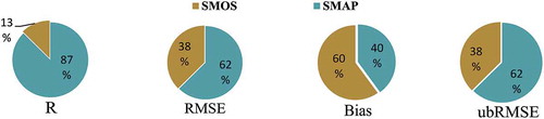
Figure 8. (a) A 1-year scatter plot for the SMAPVEX16 site formed by 81 remote sensing images of the year 2016. (b–f) T-V scatter plot for some days of the year 2016 for the corresponding network. The dotted and solid lines represent annual and daily edges, respectively
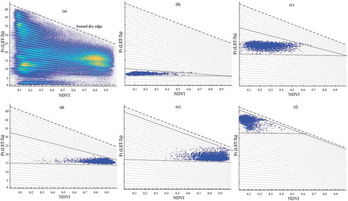
Table 3. An inspection of ground-based soil moisture, air temperature, and satellite-based vegetation conditions of 5 days that their daily scatter plots are presented in Figure 8
Figure 9. ASMIHR maps of (a): 1 May 2016, (b) 10 September 2016, (c) 15 October 2016, and (d) 18 July 2016. The corresponding maps are retrieved through the 1-year scatter plot and calculated by the annual wet and dry edge
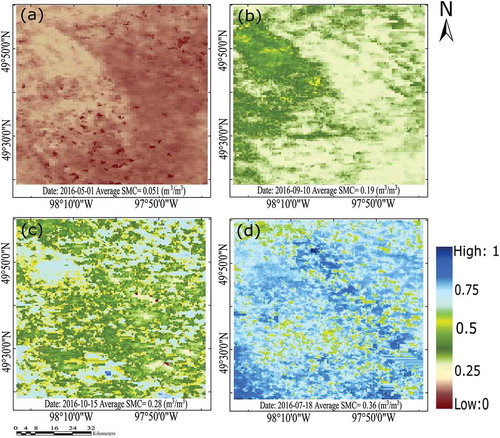
Figure 10. Time-series comparison between ASMIHR index derived from the 1-year scatter plot and in situ SMC measurements. In situ measurements and estimated ASMIHR are shown with red continues line and black circles, respectively. The average SMC values are derived from the SMC of the nine in situ stations for each day, also, the average values of the calculated index, computed over nine image pixels containing the corresponding stations
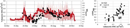
Figure 11. 36 km SMC values retrieved by SMAP mission versus the average of (a) LST, (b) Ft (LSTdaytime – Ta (10:30 a.m.)), (c) Fv (normalized NDVI), and (d) annual SMC index extracted from 1-year T-V scatter plot. Four lines in each diagram are the linear regression lines belonging to the four SMAP pixels
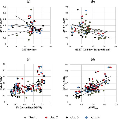
Table 4. The results of the correlation analysis between the soil moisture retrieval of four pixels of SMAP products and Fv, Ft, LST and ASMIHR over the study area
Figure 12. SMC maps derived from daily soil moisture index extracted from the 1-year T-V scatter plot alongside SMAP SMC products
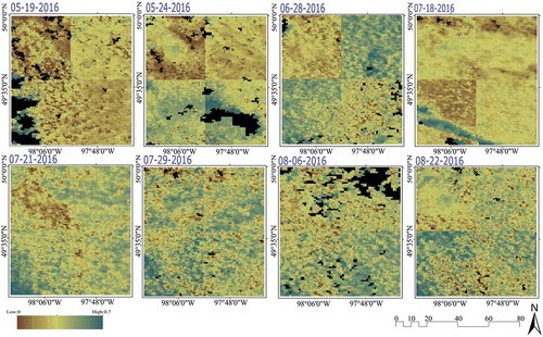
Figure 13. SMC values extracted from the 1-year scatter plot concerning the corresponding in situ SMC measurements. Each point represents an image pixel in which there is at least one in situ station
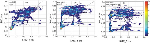
Figure 14. Correlation analysis between 5 cm soil moisture and the SMC of soil at depth (a) 20 cm, (b) 50 cm, and (c) 1 m