A workflow based on Sentinel-1 SAR data and open-source algorithms for unsupervised burned area detection in Mediterranean ecosystems

Figures & data

Figure 1. Study sites: in the top, location of the study sites in Europe and in the respective countries; in the bottom, the overviews of the two study sites (post-fire Sentinel-2 images, SWIR-NIR-Green false-color composite) where the burned areas are clearly visible (the dark-purple area in PO; the darker area in IT)

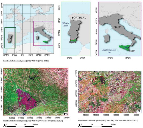
Figure 2. The workflow of the implemened approach

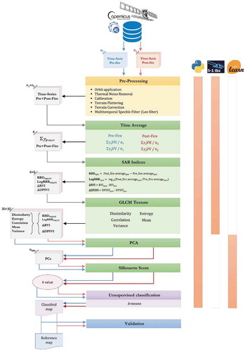
Table 1. Sentinel-1 dataset characteristics. The red line separates the images acquired before and after the fire occurrence

PO Study site				IT Study site
Mission	Orbit	Product	Sensing Date – Hour	Mission	Orbit	Product	Sensing Date – Hour
S-1B	Ascending	IW Level-1 GRDH	2018/07/01 – 18:34	S-1A	Ascending	IW Level-1 GRDH	2017/07/05 – 17:04
S-1A	Ascending		2018/07/07 – 18:35	S-1A	Descending		2017/07/06 – 05:04
S-1A	Descending		2018/07/08 – 06:35	S-1B	Descending		2017/07/12 – 05:04
S-1B	Ascending		2018/07/13 – 18:34	S-1A	Ascending		2017/07/17 – 17:04
S-1A	Ascending		2018/07/19 – 18:35	S-1B	Ascending		2017/07/18 – 16:55
S-1A	Descending		2018/07/20 – 06:35	S-1A	Ascending		2017/07/24 – 16:56
S-1B	Ascending		2018/07/25 – 18:34	S-1A	Ascending		2017/07/29 – 17:04
S-1A	Ascending		2018/07/31 – 18:35	S-1B	Ascending		2017/07/30 – 16:55
S-1A	Ascending		2018/08/12 – 18:35	S-1B	Descending		2017/08/05 – 05:04
S-1B	Ascending		2018/08/18 – 18:34	S-1A	Ascending		2017/08/17 – 16:56
S-1A	Ascending		2018/08/24 – 18:35	S-1A	Ascending		2017/08/22 – 17:04
S-1A	Descending		2018/08/25 – 06:35	S-1A	Descending		2017/08/23 – 05:04
S-1B	Ascending		2018/08/30 – 18:34	S-1B	Ascending		2017/08/23 – 16:55
				S-1A	Ascending		2017/08/29 – 16:56

Table 2. Name, group, and equation of used GLCM (Grey Level Co-occurrence Matrix) texture measures. P_i,j is the probability of values i and j occurring in adjacent pixels in the original image within the window defining the neighborhood. i and j are the labels of the columns and rows (respectively) of the GLCM: i refers to the digital number value of a target pixel; j is the digital number value of its immediate neighbor. µ is mean and σ the standard deviation

GLCM Features	Group	Equation
Dissimilarity	Contrast	$\sum _{\mathrm{i},\mathrm{j}=0}^{\mathrm{N}-1}{\mathrm{P}}_{\mathrm{i},\mathrm{j}}\left|\mathrm{i}-\mathrm{j}\right|$
Entropy	Orderliness	$\sum _{\mathrm{i},\mathrm{j}=0}^{\mathrm{N}-1}-\mathrm{l}\mathrm{n}\left({\mathrm{P}}_{\mathrm{i},\mathrm{j}}\right){\mathrm{P}}_{\mathrm{i},\mathrm{j}}$
Correlation	Statistics	$\sum _{\mathrm{i},\mathrm{j}=0}^{\mathrm{N}-1}{\mathrm{P}}_{\mathrm{i},\mathrm{j}}\left[\frac{\left(\mathrm{i}-\hspace{0.17em}{\mu }_{\mathrm{i}}\right)\left(\mathrm{i}-\hspace{0.17em}{\mu }_{\mathrm{j}}\right)}{\sqrt{\left({\sigma }_{\mathrm{i}}^2\right)\left({\sigma }_{\mathrm{j}}^2\right)}}\right]$
Mean		${\mu }_{\mathrm{i}}=\sum _{\mathrm{i},\mathrm{j}=0}^{\mathrm{N}-1}\mathrm{i}({\mathrm{P}}_{\mathrm{i},\mathrm{j}});\hspace{0.17em}{\mu }_{\mathrm{j}}=\sum _{\mathrm{i},\mathrm{j}=0}^{\mathrm{N}-1}\mathrm{j}({\mathrm{P}}_{\mathrm{i},\mathrm{j}})$
Variance		${\sigma }_{\mathrm{i}}^2=\sum _{\mathrm{i},\mathrm{j}=0}^{\mathrm{N}-1}{\mathrm{P}}_{\mathrm{i},\mathrm{j}}{\left(\mathrm{i}-{\mu }_{\mathrm{i}}\right)}^2;{\sigma }_{\mathrm{j}}^2=\sum _{\mathrm{i},\mathrm{j}=0}^{\mathrm{N}-1}{\mathrm{P}}_{\mathrm{i},\mathrm{j}}{\left(\mathrm{j}-{\mu }_{\mathrm{j}}\right)}^2$

Figure 3. The S-1 indices (RBD_VH, LogRBR_VH, ΔRVI, RBD_VV, LogRBR_VV, and ΔDPSVI) were obtained in the PO dataset pre-processing steps. For each of these indices, the GLCM (Grey Level Co-occurrence Matrix) texture features were calculated

Figure 4. The S-1 indices (RBD_VH, LogRBR_VH, ΔRVI, RBD_VV, LogRBR_VV and ΔDPSVI) were obtained in the IT dataset pre-processing steps. For each of these indices, the GLCM (Grey Level Co-occurrence Matrix) texture features were calculated

Figure 5. The cumulative variance explained by the principal components (PCs) for the PO study site. The red line identifies the first PCs that reached a cumulative variance of 0.99

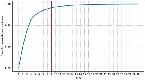
Figure 6. The cumulative variance explained by the principal components (PCs) for the IT study site. The red line identifies the first PCs that reached a cumulative variance of 0.99

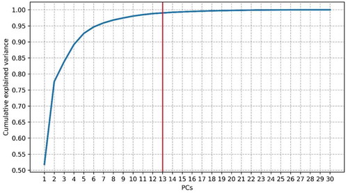
Figure 7. Silhouette score values, for the PO dataset, for a k-space range (k values) between 2 and 20

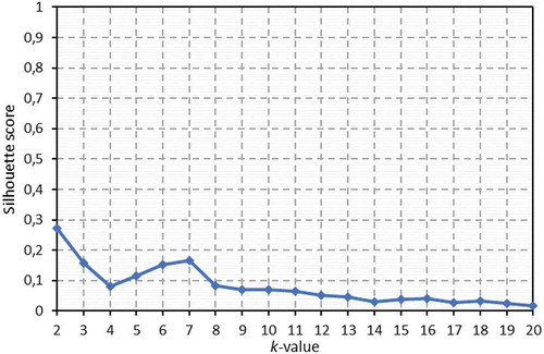
Figure 8. Silhouette score values, for the IT dataset, for a k-space range (k values) between 2 and 20

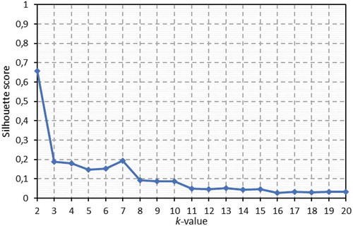
Figure 9. Classification results, showing the seven classes for both study areas. The blue clusters (classes 3–4 in the PO, and 6 in IT) represent the burned areas’ classes

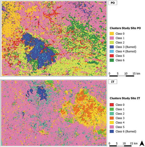
Figure 10. The figure shows the distribution of the mean value of each radar index across all six classes for both study sites (PO and IT) (at the top). At the bottom, boxplots of indices values for each class are reported (the white rhombus marker indicates the mean values)

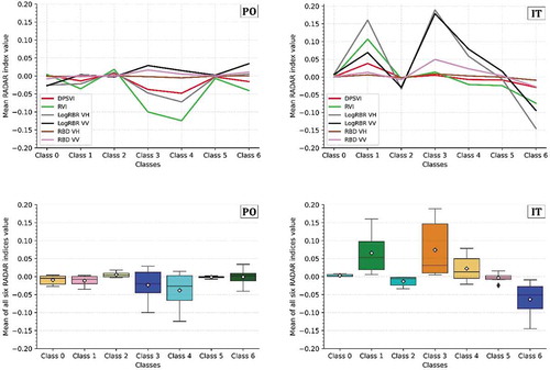
Table 3. Distribution of each dataset’s pixels and the three accuracy categories (true positive, TP; false negative, FN; false positive, FP) for both study sites (PO and IT)

GLCM Features	PO	IT
TP	80.47%	85.57%
FP	19.95%	14.94%
FN	19.53%	14.43%

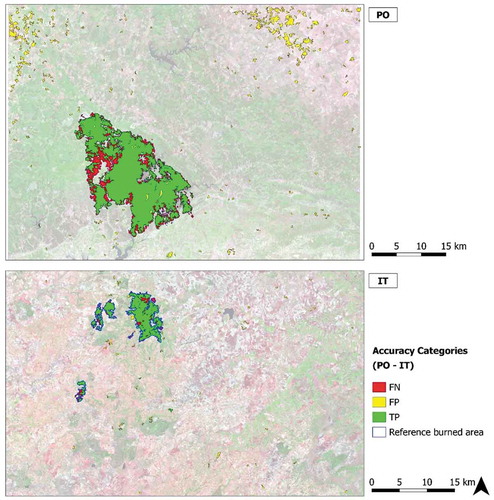
Figure 11. The maps show the spatial distribution of the three accuracy categories, true positive (TP, green), false positive (FP, yellow), false negative (FN), for IT and PO study sites, using the reference layer (blue) derived from S-2 data

Data availability statement

The implemented process code is available online at https://doi.org/10.5281/zenodo.4556927.