Figures & data
Table 1. Data list and information.
Figure 1. The framework of mapping temporal population dynamics.
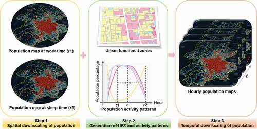
Figure 2. The workflow of generating baseline population maps during sleep and work times using the dasymetric method. From ① to ②generation of baseline population (sleep time) based on residential building height in urban areas and VIIRS NTL intensity in rural areas, respectively. From ③ to ⑤generation of baseline population (work time) based on nonresidential population and nonresidential building height.
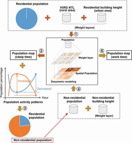
Figure 3. Flow chart of generating urban functional zones (UFZ). Generating parcels (a); Deriving parcel attributes (b); and generation and accuracy evaluation of UFZ (c).
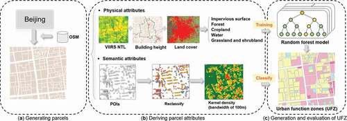
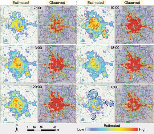
Figure 4. Illustration of proposed framework for temporal population downscaling based on two baseline populations and population activity patterns. Note that the population on the road was changing over time.
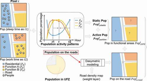
Figure 5. Spatial patterns of derived baseline population maps. Populations during sleep time (a) and work time (b); Population density map at the administrative unit of level 4 during sleep time (c) and work time (d).
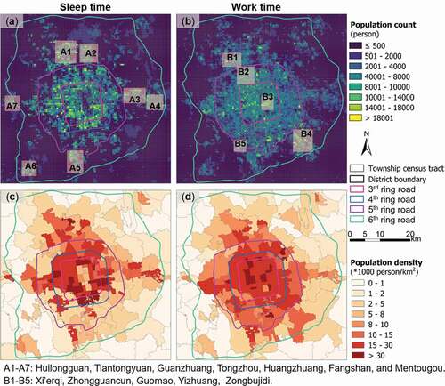
Figure 6. Evaluation of derived baseline populations using the reference data. Comparison of the derived population with census data during sleep time across ring areas (a) and with Baidu LBS data collected at 0:00 at the administrative unit of level 4 (b); as well as the comparison of the derived population during work time with Baidu LBS data collected at 11:00 at the administrative unit of level 4 (c).
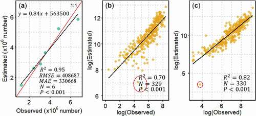
Table 2. Confusion matrix in categorizing UFZ.
Figure 7. Total operating characteristic (TOC) for the performance of RF in the classification of UFZ. Note that the transportation class only includes large public transportation hubs (e.g. railway station and airport) in this paper.
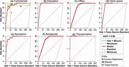
Figure 8. Urban functional zones of Beijing in 2015. An overview (a); close-up within the red box showing the city center of Beijing (b); area percentages of different functional types within each ring area (c).
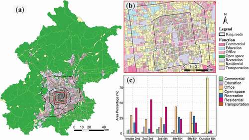
Figure 9. The estimated patterns of human activities.
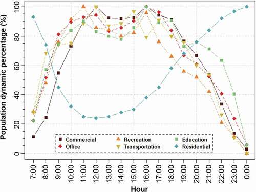
Figure 10. Comparison of population heat maps between our estimations and that from Baidu Maps collected on 24 September 2020. Areas marked with red dash circles are aggregated nonresidential regions. Areas marked with black dash circles are aggregated residential regions.