Analyzing spatial variability of drivers of coastal wetland loss in the northern Gulf of Mexico using Bayesian multi-level models

Figures & data

Figure 1. The study area with two spatial scales: watersheds using Hydrological Unit Codes 4 (HUC4) watershed boundaries shown in blue to purple, and sites of wetland loss shown as yellow dots (see enlarged right panel – A). Darker colors of blue or purple indicate higher 10-year summer median of streamflow discharge (ft³/sec) derived from the USGS streamflow data. Subplot on the bottom (B) shows the number of sites within each watershed. Watershed numbers on the map correspond to the watershed numbers on the subplot. Official HUC4 designations are: 1) Southern Florida (S FL), 2) Peace-Tampa Bay (W FL), 3) Suwannee (Big Bend FL), 4) Ochlockonee (E PH FL), 5) Apalachicola (C PH FL), 6) Choctawhatchee-Escambia (W PH FL), 7) Mobile-Tombigbee(Mob AL), 8) Pascagoula (MS Coast), 9) Mississippi Delta (MS Delta), 10) Louisiana Coastal (W LA), 11) Galveston Bay-San Jacinto (E TX), 12) Lower Colorado-San Bernard Coastal (C TX), 13) Central Texas Coastal (W TX), and 14) Nueces-Southwestern Texas Coastal (S TX) from east to west

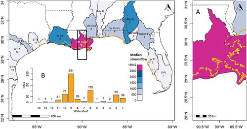
Figure 2. Boxplots of covariates and response variable for each watershed. The thick horizontal line shows the median, the wide box shows the upper and lower quartiles (25 and 75%), and the dotted “whiskers” show the distribution from the quartiles to the 1.5 interquartile range. RSLR denotes relative sea-level rise, and NDVI denotes normalized difference vegetation index from Landsat-5 imagery. Note: Landsat-5 images have seven spectral bands: band 1 = blue; band 2 = green; band 3 = red; band 4 = near-infrared (NIR); band 5 = shortwave infrared (SWIR 1); band 6 = thermal; band 7 = SWIR 2 with a revisit time of 16 days and a spatial resolution of 30 meters (m) except the thermal band with a spatial resolution of 120 m

Figure 3. Structure of the Bayesian multi-level model used to identify the biogeophysical variables that affected wetland loss. Wetland loss was a function of geophysical properties and a vegetation index, the effects of which may $(covariatesk+1\dots m)$ or may not $(covariates1\dots k)$ vary in different watersheds. For the covariates that we assumed to affect wetland loss by watershed, we sampled their associated parameters for each watershed from the parameters at the scale of the entire study area (global scale). $m=totalnumberofcovariates$, $k=numberofcovariates$, the effects of which on wetland loss did not vary in different watersheds. $\beta s=interceptandparameters$ associated with normalized covariates $(C)$, $\alpha s=thehyper-parameters$ from which $\beta s$ were sampled, $W=logarithmofarealwetlandloss$, $i=watersheds$, and j = sites. Refer to the main text for formulas of different equations identified in this figure

Table 1. Results of the best model candidates in which ΔDIC is less than 2 out of the 484 models for areal wetland loss. ${\beta }_0$ denotes intercept, RSLR denotes relative sea level rise, WH denotes wave height, TR denotes tidal range, CS denotes coastal slope, and NDVI denotes normalized different vegetation index. DIC denotes deviance information criterion and PPL denotes posterior predictive loss. Both DIC and PPL were applied in the model selection. The lower the DIC and PPL, the better the model predictions. The model numbers under the significant covariates columns denote watersheds identified in Figure 1 where that particular covariate had an effect different from zero (95% credible intervals do not overlap 0) on coastal wetland loss. An X mark under a covariate represents that covariate was included in the model

	Covariates effects of which do not vary across watersheds						Covariates effects of which vary across watersheds						Model metrics		Significant covariates
Model #	RSLR	NDVI	WH	TR	CS	${\beta }_0$	RSLR	NDVI	WH	TR	CS	${\beta }_0$	$\mathrm{\Delta }\mathrm{D}\mathrm{I}\mathrm{C}$	PPL	RSLR	NDVI	WH	TR	CS	${\beta }_0$
58							X		X	X		X	0.00	952.27	6,8,10		1,9	1,8,9		8
146							X		X	X	X	X	0.08	953.16	6,8,10		1,9	1,9		9
145					X		X		X	X		X	1.46	968.74	6,8,10		1,9	1,9		8,11
241		X					X		X	X	X	X	1.56	969.78	6,8,10		1,9	1,9		8
161		X					X		X	X		X	1.65	968.85	6,8,10		1,9	1,9		8

Table 2. Summary of the coefficients for the covariates selected in the best areal wetland loss model #58. We grouped rows by watershed (denoted by 1 to 14 within model). We highlighted the covariate with the largest absolute median for each watershed. Sd denotes standard deviation, and 2.5% and 97.5% denote 2.5% quantile and 97.5% quantile. Covariate abbreviations defined in Table 1

	mean	sd	2.5%	median	97.5%
bRSLR[1]	−0.41	0.48	−1.37	−0.4	0.51
bTR[1]	−0.71	0.29	−1.28	−0.71	−0.16
bWH[1]	−0.76	0.27	−1.3	−0.76	−0.22
bRSLR[2]	1.02	0.7	−0.32	1	2.46
bTR[2]	0.09	0.26	−0.42	0.09	0.6
bWH[2]	−0.53	0.43	−1.39	−0.52	0.28
bRSLR[3]	0.47	0.93	−1.49	0.5	2.24
bTR[3]	0.11	0.42	−0.74	0.11	0.93
bWH[3]	−0.25	0.79	−1.87	−0.23	1.28
bRSLR[4]	0.23	0.93	−1.79	0.29	1.93
bTR[4]	−0.22	0.45	−1.14	−0.21	0.65
bWH[4]	−0.45	0.77	−2.07	−0.41	0.99
bRSLR[5]	0.82	0.73	−0.6	0.81	2.28
bTR[5]	−0.37	0.98	−2.37	−0.36	1.57
bWH[5]	−0.17	0.8	−1.8	−0.16	1.38
bRSLR[6]	0.93	0.25	0.45	0.93	1.42
bTR[6]	−0.02	0.16	−0.33	−0.02	0.3
bWH[6]	0.02	0.31	−0.59	0.02	0.63
bRSLR[7]	0.77	0.53	−0.26	0.76	1.82
bTR[7]	−0.54	0.89	−2.39	−0.51	1.16
bWH[7]	−0.11	0.62	−1.35	−0.11	1.1
bRSLR[8]	1.12	0.53	0.1	1.11	2.19
bTR[8]	−1.32	0.65	−2.7	−1.28	−0.12
bWH[8]	−0.44	0.59	−1.64	−0.42	0.71
bRSLR[9]	1.24	0.39	0.48	1.24	2.02
bTR[9]	0.15	0.32	−0.47	0.14	0.78
bWH[9]	0.1	0.29	−0.47	0.1	0.67
bRSLR[10]	0.5	0.3	−0.11	0.5	1.08
bTR[10]	−1.34	0.36	−2.06	−1.34	−0.64
bWH[10]	0.62	0.1	0.43	0.62	0.81
bRSLR[11]	0.27	0.97	−1.84	0.32	2.03
bTR[11]	0.85	0.8	−0.55	0.8	2.56
bWH[11]	0.07	0.3	−0.52	0.07	0.65
bRSLR[12]	0.64	0.97	−1.33	0.65	2.55
bTR[12]	−0.3	0.87	−2.01	−0.31	1.44
bWH[12]	−0.14	0.7	−1.54	−0.13	1.23
bRSLR[13]	0.5	0.89	−1.33	0.52	2.25
bTR[13]	−0.51	0.46	−1.42	−0.51	0.41
bWH[13]	0.25	0.54	−0.8	0.24	1.35
bRSLR[14]	0.88	0.85	−0.78	0.86	2.62
bTR[14]	−0.37	0.98	−2.36	−0.36	1.58
bWH[14]	0.04	0.74	−1.42	0.03	1.54

Figure 4. Maps of the medians of the coefficients in the best areal wetland loss model (#58) at the watershed scale (note each watershed has multiple coastal wetland sites). We standardized the covariates so that the coefficients were comparable both between watersheds, and between covariates. In the inset plots, a dot represented the median of the parameter posterior for each watershed, with associated 95% credible interval represented by a line crossing the median. A solid dot indicated a positive or negative effect of the covariate on coastal wetland loss for the given watershed (95% credible interval does not contain 0), and an unfilled dot indicated an effect not different from 0. RSLR denotes relative sea-level rise, WH denotes wave height, TR denotes tidal range, and b0 denotes intercept of the site-scale submodel (Eq. 3)

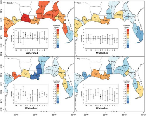
Table 3. Comparison of models with streamflow and/or land use/land cover as covariates at the watershed scale for intercept to the best model (Model #58) without consideration of streamflow and/or land use/land cover for intercept. (SF denotes streamflow (ft³/sec), DV denotes percent developed areas, FR denotes percent forest areas, 2.5% and 97.5% denote 2.5% quantile and 97.5% quantile of the parameters, k₁ denotes the coefficient for streamflow, k₂ denotes the coefficient for percent forest areas, and k₃ denotes the coefficient for percent developed areas)

	Model metrics	Parameters
Model #	$\mathrm{\Delta }\mathrm{D}\mathrm{I}\mathrm{C}$	Name	2.5%	Median	97.5%
Model 58	0.00	No covariates at the watershed scale
SF	−0.75	k1(SF)	−0.292	0.351	1.020
SF, FR, DV	−1.21	k1(SF)	−0.289	0.388	1.082
		k2(FR)	−1.468	−0.590	0.356
		k3(DV)	−1.181	−0.336	0.517

Data Availability Statement

Data and code for analysis can be found at the project’s GitHub page at http://github.com/ecospatial/NAS_2016. We have also created a READ.ME file for users and the complete data archiving is underway.