Recent trends in the timing of the growing season in New Zealand’s natural and semi-natural grasslands

Figures & data

Figure 1. Study area: The Clutha/Mata-Au river catchment, New Zealand showing the spatial distribution of the three grassland types (alpine grass/herbfield, Tall Tussock and low producing) investigated in this study (LCDB-v4.1 2015). The average Normalized Difference Vegetation Index (NDVI) in the catchment during 2001–2016 was calculated from a MODIS time series (see methods)

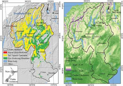
Table 1. The five indices used to quantify growing season phenology in this study. The mDOY is the modified day of year, where mDOY 1 is 1st July of last year and mDOY 365 is 30th June of this year

No	Index	Abbreviation	Description
1	Start of season	SOS	Start of the growing season: the day where 50% of the year’s peak NDVI is reached for the first time, described by mDOY.
2	End of season	EOS	End of the growing season: the day at which NDVI falls under 50% of the peak NDVI, described by mDOY.
3	Length of season	LOS	Length of growing season: the time period in days between start and end of season, described by days.
4	Peak of season	POS	The peak of growing season, the day when the peak NDVI is reached, described by mDOY.
5	Peak day NDVI	P-NDVI	The fitted NDVI value on the day of the Peak of season

Figure 2. Calculation of five phenological indices. Taking one pixel (see its location in the inset map) from the 16-year NDVI time series for example: the blue line is the raw NDVI data. The black curve is the asymmetric Gaussian function fitted values. Growing phenological indices were derived from the fitted values. Inset shows how the five phenological indices were calculated. SOS = Start of season, EOS = end of season, LOS = length of season, POS = peak of season, P-NDVI = peak day NDVI. We used a modified day-of-year (mDOY) to describe growth phenology in the southern hemisphere. A growing year starts from 1st July of last year and ends on 30th June of this year (mDOY 1 = 1st July of last year, mDOY 365 = 30st June)

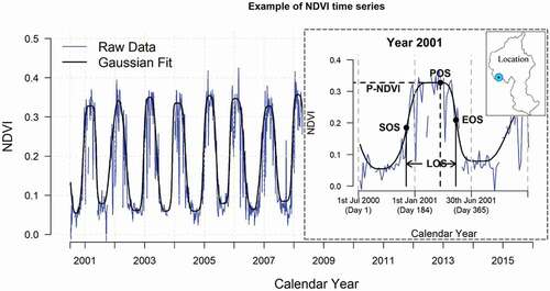
Table 2. Summary statistics (average, standard deviation) of the five phenological indices for the three grassland types for the study period 2001–2016. mDOY refers to the modified day of year with mDOY = 1 being 1^st July (see Table 1 and methods)

Phenological Index	Alpine		Tall Tussock		Low Producing
	Mean	SD.	Mean	SD.	Mean	SD.
Start (SOS, mDOY)	149.9	31.96	119.4	28.10	93.4	24.76
End (EOS, mDOY)	313.6	23.75	314.1	21.34	275.3	45.86
Length (LOS, days)	163.7	39.82	194.7	32.49	181.9	40.47
Peak (POS, mDOY)	233.8	20.27	219.7	19.92	182.7	31.90
Peak NDVI (P-NDVI)	0.33	0.109	0.47	0.078	0.59	0.088

Table 3. Temporal trends of five phenological indices during the study period 2001–2016. We calculated the OLS models of phenological indices against year for each single MODIS pixel, so each pixel has its own temporal trends quantified by the estimated values (slopes) of OLS models. The median (med) and extremes (max, min) are based on individual pixels in each grassland type, and the med* is the median of those pixels which showed a significant temporal trend (p < 0.05)

Phenological index	Grassland type	Med	Max	Min	Med*
Start (SOS, days/year)	Alpine	−0.72	2.43	−5.73	−2.10
	Tall Tussock	−0.60	5.80	−6.83	−1.64
	Low Producing	−0.88	10.82	−11.99	−1.47
End (EOS, days/year)	Alpine	−0.45	5.27	−4.60	−1.35
	Tall Tussock	−0.04	5.76	−6.48	1.36
	Low Producing	−0.04	12.07	−9.03	−0.71
Length (LOS, days/year)	Alpine	0.32	9.76	−3.99	2.81
	Tall Tussock	0.52	9.14	−6.05	2.73
	Low Producing	0.71	12.65	−10.69	2.56
Peak (POS, days/year)	Alpine	−0.63	1.98	−3.05	−1.54
	Tall Tussock	−0.32	4.11	−4.41	−1.34
	Low Producing	−0.66	10.26	−9.00	−2.24
Peak NDVI (P-NDVI, 10^−2/year)	Alpine	0.05	0.82	−1.24	0.24
	Tall Tussock	0.02	1.61	−1.49	0.16
	Low Producing	−0.04	2.54	−1.90	−0.20

Figure 3. The averages of phenological indices for the time period of 2001–2016. The start (a), peak (b) and end (c) days of growing season were described by a modified day of year (mDOY, which begins on 1st July of last year and ends on 30th June in this year). The length (d) of season was in units of days. The peak NDVI (e) ranged from 0.1–0.8 with higher values indicating more active vegetation

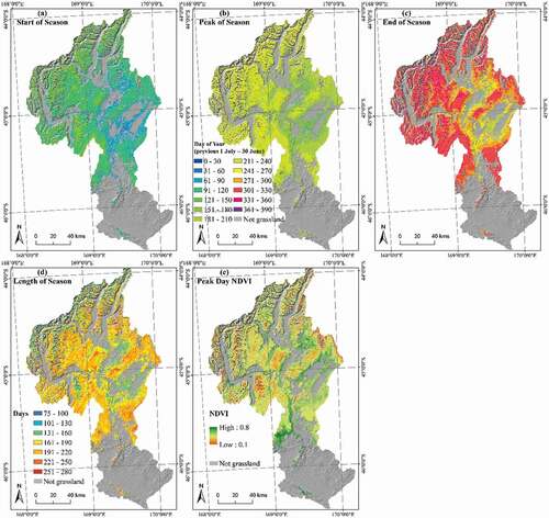
Figure 4. The distributions of the trends in each growth phenological index in each grassland type. ALP: Alpine grassland; TSK: Tall Tussock grassland; LPG: Low Producing grassland. The dotted vertical line in each panel separates the positive (red) and negative (blue) trends. The darker colored region indicates the significant (p < 0.05) trends. The proportion values in each panel show the percentages of positive/negative trends in all pixels, and the percentages in round brackets are the significant (p < 0.05) proportions of pixels

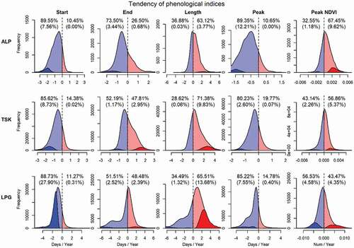
Figure 5. Temporal trends in the five growth phenological indices in the past 16 years (2001–2016). For start (a), End (b), Peak (c) and length (d) of season, the red (p ≤ 0.05) and coral (p > 0.05) colors represent the grassland with positive phenological trends (delayed start, end and peak of season, or prolonged length of season), and the blue (p ≤ 0.05) and turquoise (p > 0.05) colors illustrate the grassland with negative phenological trends (advanced start, end and peak of season, or shortened length of season). For peak NDVI (e), the green regions show an increasing trend in NDVI and dark-green color indicates significant, while the yellow areas show a decreasing trend in NDVI and brown color means significant

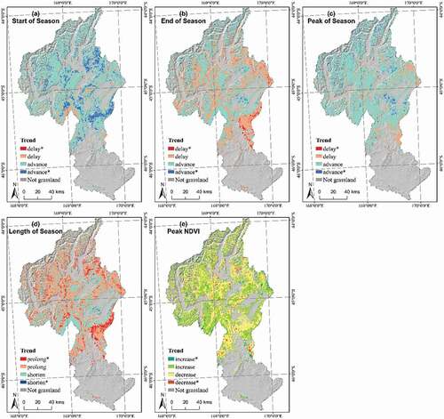
Table 4. Correlations between the five phenological indices and eight climatic factors. Values indicate the average slope (β) of OLS model of the pixels showing a significant linear relationships (t-test p < 0.05), and the percentages under the slopes indicate the proportions of the pixels in each grassland type showing a significant correlation

Index	Grass Type	ETmp	MSLP	Rad	Rain	RH	TMax	Tmin	Wind
Start SOS (days /unit)	Alp	−17.65	−3.35	−0.43	0.14	−4.71	−4.46	5.82	4.02
		1%	78%	1%	21%	2%	2%	1%	1%
	Tsk	−23.58	−3.05	−0.09	0.16	0.91	4.62	7.50	−13.20
		3%	64%	4%	26%	3%	1%	1%	4%
	Lpg	−17.49	−2.25	−0.06	0.16	4.95	−3.09	4.32	−16.04
		8%	25%	9%	23%	4%	3%	5%	8%
End EOS (days /unit)	Alp	8.15	1.80	0.05	0.10	−3.80	−6.20	3.97	25.10
		16%	2%	29%	2%	2%	1%	18%	4%
	Tsk	12.23	NA	0.04	0.35	−4.25	−2.56	2.83	28.79
		19%	0%	16%	2%	4%	<1%	7%	2%
	Lpg	−33.43	1.76	0.01	0.46	8.17	−3.39	4.86	13.27
		6%	7%	4%	32%	4%	2%	1%	4%
Length LOS (days /unit)	Alp	19.54	10.14	0.02	−0.04	5.23	−2.99	−8.53	21.94
		5%	11%	1%	1%	2%	1%	2%	5%
	Tsk	36.42	10.65	0.04	−0.05	−1.50	−3.07	−7.58	37.36
		9%	13%	1%	2%	7%	<1%	4%	12%
	Lpg	−5.35	11.44	−0.02	0.18	−3.11	1.64	−0.09	24.06
		10%	16%	3%	15%	2%	1%	6%	11%
Peak Day POS (days /unit)	Alp	−10.34	−2.10	0.07	0.13	−2.61	4.38	−0.30	18.48
		1%	1%	13%	4%	2%	2%	2%	4%
	Tsk	−12.67	3.68	0.05	0.15	−2.31	1.26	−6.43	25.42
		3%	<1%	5%	11%	5%	<1%	6%	1%
	Lpg	−10.87	−1.25	0.02	0.28	0.04	−2.54	−1.34	−1.87
		3%	3%	1%	40%	2%	1%	3%	3%
P-NDVI (1/unit)	Alp	−1.32 E-02	1.15 E-02	2.23 E-05	5.37 E-06	−6.68 E-04	3.58 E-03	−4.12 E-04	−1.81 E-03
		6%	26%	1%	5%	6%	16%	3%	2%
	Tsk	−1.01 E-02	5.66 E-03	−5.60 E-05	1.87 E-04	8.72 E-03	2.94 E-03	9.56 E-03	−5.32 E-02
		14%	9%	3%	7%	30%	17%	7%	12%
	Lpg	−1.32 E-02	−4.38 E-03	−4.54 E-05	2.23 E-04	1.22 E-02	−4.63 E-03	1.22 E-02	−6.78 E-02
		9%	6%	5%	19%	28%	4%	11%	16%

Abbreviations: ETmp: 10 cm earth temperature [°C], MSLP: mean sea level pressure [hPa], Rad: solar radiation [MJ/m²/day], Rain: rainfall [mm], RH: relative humidity [%], Tmax, Tmin: maximum, minimum temperature [°C], Wind: wind speed [m/s]. Alp: Alpine grassland, Tsk: Tall Tussock grassland, Lpg: Low Producing grassland.

Figure A1 The trends of the five phenological indices in three grassland types during 2001–2016. The lines show the extremes and median of trends of five phenology indices in three grassland types. The red/blue solid lines are the most positive/negative tendency during the 16 years, and the dotted red/blue lines are for those two pixels. The gray line represents the median trend slopes in each scenario.

Irrigation regions in the study area (Clutha catchment). Data obtained from ministry for the environment, New Zealand (https://www.mfe.govt.nz/fresh-water/freshwater-guidance-and-guidelines/irrigated-land-new-zealand).

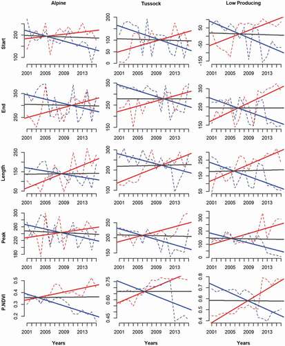
Figure A2. (Continued)

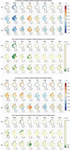
Figure A2. (Continued)

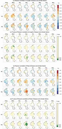
Figure A2. The spatial patterns of the correlations between annual growth phenological indices and climatic factors quantified by Pearson correlation coefficients (PCCs). The reddish colors represent positive relationships, while the blues mean negative correlations. The dark green colors indicate significant correlations (p < 0.05 in ANOVA test).

Abbreviations: ETmp, 10 cm earth temperature; MSLP, mean sea level pressure; Rad, solar radiation; Rain, rainfall; RH, relative humidity; Tmax, maximum temperature; Tmin, minimum temperature; Wind, wind speed; alp, Alpine grassland; tsk, Tall Tussock grassland; lpg, Low Producing grassland

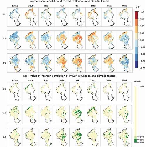
Figure A3. The trend of eight climate factors during the 2001–2016 study period. In each climate factor’s panel, the left map shows its trend of annual changes, and the map on the right shows the statistical significance (p-value) of its changing trend during 2001–2016.

Abbreviations: ETmp, 10 cm earth temperature (degC/year); MSLP, mean sea level pressure (hPa/year); Rad, solar radiation (MJ/m2/year); Rain, rainfall (mm/year); RH, relative humidity (%/year); Tmax, maximum temperature (degC/year); Tmin, minimum temperature (degC/year); Wind, wind speed (m/s/year)

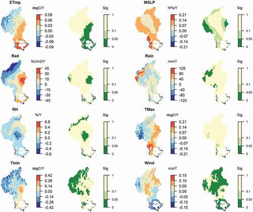
Figure A4. The averages of eight climatic factors in the Clutha river catchment in 2001–2016.

Abbreviations: ETmp: 10 cm earth temperature; MSLP: mean sea level pressure; Rad: solar radiation; Rain: rainfall; RH: relative humidity; Tmax, Tmin: maximum and minimum temperatures; Wind: wind speed

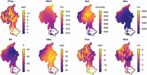
Figure A5. Irrigation regions in the study area (Clutha catchment). Data obtained from ministry for the environment, New Zealand

(https://www.mfe.govt.nz/fresh-water/freshwater-guidance-and-guidelines/irrigated-land-new-zealand)

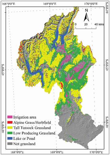
Table A1. Definitions of grassland types in LCDB v4.1

Class Name	Definition
Alpine Grass/Herbfield	Typically sparse communities above the actual or theoretical treeline dominated by herbaceous cushion, mat, turf, and rosette plants and lichens. Grasses are a minor or infrequent component, whereas stones, boulders and bare rock are usually conspicuous.
Tall Tussock Grassland	Indigenous snow tussocks in mainly alpine mountain-lands and red tussock in the central North Island and locally in poorly-drained valley floors, terraces and basins of both islands.
Low Producing Grassland	Exotic sward grassland and indigenous short tussock grassland of poor pastoral quality reflecting lower soil fertility and extensive grazing management or non-agricultural use. Browntop, sweet vernal, danthonia, fescue and Yorkshire fog dominate, with indigenous short tussocks (hard tussock, blue tussock and silver tussock) common in the eastern South Island and locally elsewhere.

LCDB-v4.1. 2015. “Land Cover Database Version 4.1.” The Land Resource Information Systems Portal and scinfo.org.nz, Accessed June 16. https://lris.scinfo.org.nz/layer/423-lcdb-v41-land-cover-database-version-41-mainland-new-zealand.

 Google Scholar

Data availability statement

The processed MODIS NDVI data that support the findings of this study are available from the co-author Pascal Sirguey [email protected] upon reasonable request. The original MODIS imagery is available at https://modis.gsfc.nasa.gov/data/dataprod/.

The climate data (VCSN) that support the findings of this study are openly available in NIWA at https://data.niwa.co.nz.