
Figures & data
Figure 1. Methodological approach of this study. Orange parallelepipeds indicate input remote sensing data; yellow boxes symbolize processing steps and red parallelepipeds indicate input data for the random forests. Light blue ovals symbolize the intermediate results and the blue oval indicate the end result.

Figure 2. Study area with the training area (northern part of the Netherlands; blue), the validation areas (Zeeland, Noord-Brabant, Limburg; brown) and the test area (Groningen; green)
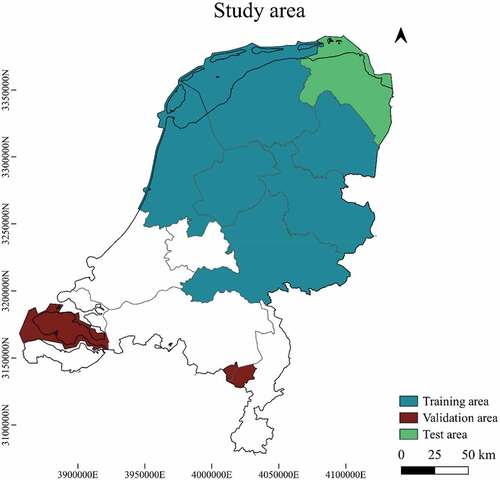
Table 1. Overview of the objects per land cover category in the training dataset.
Table 2. Satellite imagery used in this study.
Figure 3. RGB Sentinel-2 imagery showing a part of the test area with the location of solar park panels on top. Backscatter imagery of the VV mode from March 2021 in the bottom.
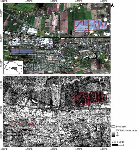
Table 3. The number of objects in the oversampled, subsampled, and land cover categories training datasets, after data augmentation.
Table 4. Validation results for different RF models trained on datasets with oversampled yes/no categories.
Figure 4. RGB Sentinel-2 imagery showing a part of the test area. Firstly, Sentinel-2 10 m resolution imagery was segmented with the SNIC algorithm (a). Secondly, the objects were classified with an RF model (b). To facilitate interpretation, true negatives are not shown on the map.
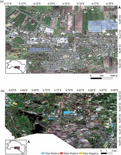
Figure 5. Variable importance plot of the RF model trained on an oversampled dataset and using the 10- and 20-meter resolution (green, blue, red, NIR, NDVI, NDWI, Red edge and SWIR) Sentinel-2 bands in combination with VV and VH backscatter properties from Sentinel-1 imagery as explanatory variables.
Figure 6. Spectral reflectance curves of included land cover categories based on the 10 and 20 m resolution bands of Sentinel-2 imagery from March 2021.
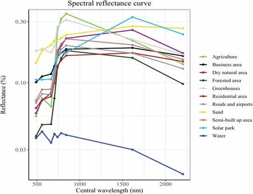
Figure 7. Variable importance plot showing the mean SHAP values over all observations of the RF model trained on an oversampled dataset and using the 10- and 20-meter resolution (green, blue, red, NIR, NDVI, NDWI, Red edge and SWIR) Sentinel-2 bands in combination with VV and VH backscatter properties from Sentinel-1 imagery as explanatory variables.
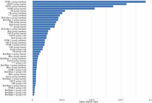
Figure 8. ROC curve of the validation dataset classified by the RF model trained on an oversampled dataset and using the 10- and 20-meter resolution (green, blue, red, NIR, NDVI, NDWI, Red edge and SWIR) Sentinel-2 bands in combination with VV and VH backscatter properties from Sentinel-1 imagery as explanatory variables.
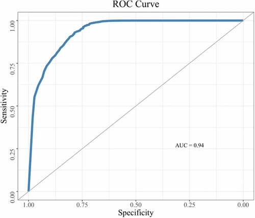
Table 5. The methodology, and the accuracy metrics and statics of this study and previous studies addressing solar panel detection (OA: overall accuracy; PA: producer accuracy; UA: user accuracy).
Figure A1. Land cover map with the objects from the Bestand Bodemgebruik and the segmented solar park objects. The map covers a part of the test area.
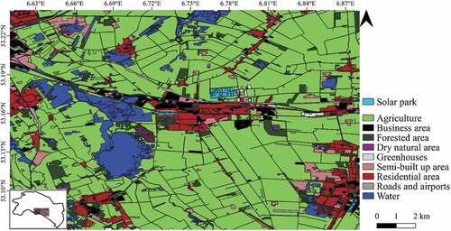
Table A2. Validation results for different RF models trained on datasets with subsampled yes/no categories.
Table A1. Accuracies and metrics of the validation dataset classified by RF models trained on datasets with land cover categories.
Data availability statement
Replication data and codes used to generate the results presented in this paper can be obtained from https://doi.org/10.34894/5NYLSG