
Figures & data
Figure 1. Location of the study area of Hangzhou, and the Landsat image collection. (a) Mosaic true color image (R: 3, G: 2, B:1) of the study area from four synthetic Landsat images for 1 July 2019. (b) Classification map for 2019 (overall accuracy: 85.7%, Kappa coefficient: 0.82) illustrating the main land use and cover types. (c) Distribution of all available Landsat images collected from scene 119/39.
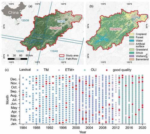
Figure 2. General framework for mapping the time-series Remote Sensing–based Ecological Index (ts-RSEI).
Figure 3. Mechanism of Continuous Change Detection and the Classification (CCDC) algorithm. (a1–a3) Process of capturing Land Use and Cover Changes (LUCC) using a piecewise linear harmonic model, using the reflectance of the SWIR1 band as an example. The green and blue curves correspond to different model pieces before and after LUCC. (b1–b3) Google Earth history snapshots acquired from the periods labeled by the red rectangles in (a1–a3). The yellow pin corresponds to the location where the CCDC algorithm was applied. (c1–c2) Synthetic Landsat images for 1 July 2010 and 1 July 2018, generated by model coefficients. (d1–d2) Classification maps for Jul.1, 2010 and Jul.1, 2018, generated by XGBoost classifiers. The red cross corresponds to the pixel where the CCDC algorithm applies.
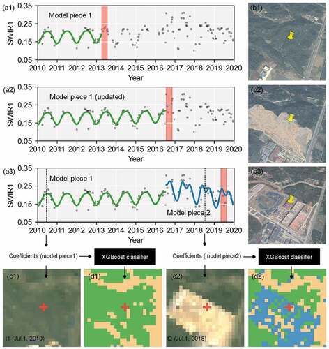
Figure 4. Absolute difference distributions for the pairwise RSEI calculated using real and synthetic Landsat images. The absolute difference distributions for the overall area (a) and main land use and cover types (b) are calculated using the pairwise RSEI derived from real Landsat images with different timespans. The monthly absolute difference distributions for the overall area (c) and main land use and cover types (d) are calculated using the pairwise RSEI derived from real and synthetic Landsat images. The mean absolute differences (MAD) are labeled with dashed lines: blue for the overall area, green for forest, yellow for cropland, and red for artificial surfaces. Gray numbers denote the image numbers used for calculation.
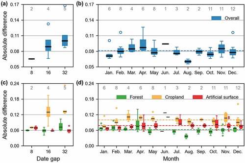
Figure 5. Differences in pairwise RSEI between real Landsat images with different timespans. The first and second columns are the RSEIs calculated for the real Landsat images for two adjacent periods. The timespan between the first and second columns increases by rows, 8 days for (a), 16 days for (b), and 32 days for (c). The third column shows the RSEI differences between the first and second columns, with the outstanding differences labeled with land use and cover type. The fourth column shows a histogram of the RSEI differences and the Mean Absolute Difference (MAD).
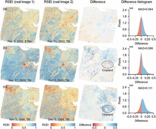
Figure 6. Temporal and spatial validation of ts-RSEI maps. Temporal validation was conducted for three typical sites – a built-up area (a), cropland (b), and forest (c) – before and after Land Use and Cover Change (LUCC). Sub-figures 1–3 show Google Earth snapshots before and after LUCC; and sub-figures 4–6 show ts-RSEI maps before and after the LUCC. Spatial validation was conducted on the three urban parks (and adjacent areas) of Xixi, Xihu, and Banshan. Sub-figures 1–3 and 4–6 show Google Earth snapshots and ts-RSEI maps, respectively.
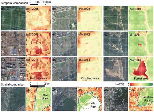
Figure 7. Correlations between the ts-RSEI and the Impervious Surface Percentage (ISP) for the years 2000 (a), 2005 (b), and 2010 (c).
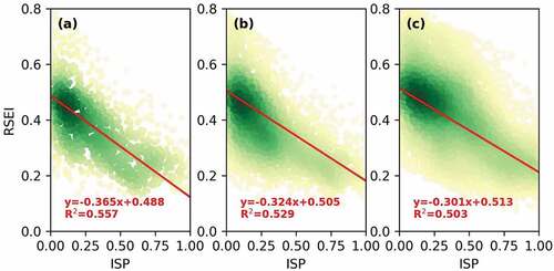
Figure 8. Differences between the RSEI and ts-RSEI from real and synthetic Landsat images with the same date. The first and second columns are the RSEIs and ts-RSEIs calculated for real and synthetic Landsat images. Difference between the RSEI and ts-RSEI by season and decade, including spring in the 1980s (a), summer in the 2000s (b), autumn in the 2010s (c), and winter in the 1990s (d). The third column shows the differences between the first and second columns, with the outstanding differences labeled with the land use and cover type. The fourth column shows a histogram of the differences and the Mean Absolute Difference (MAD).
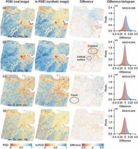
Figure 9. Spatial divergence of ecological quality in Hangzhou during 1986–2019 evaluated by annual ts-RSEI. For each annual ts-RSEI, the date of Jul. 1 of the corresponding year was used.
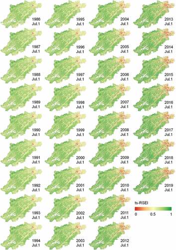
Figure 10. Annual changes in ecological quality in Hangzhou during 1986–2019. The mean values (points) and standard deviations (error bars) of the ts-RSEI are used to depict the ecological quality. Key turning points in ecological quality are labeled with the mean ts-RSEI value. Changes in ecological quality are evaluated for the overall area (a) and the main land use and cover types, including forest (b), cropland (c), and artificial surfaces (d). The area percentages for the main land use and cover types are shown as gray bars.
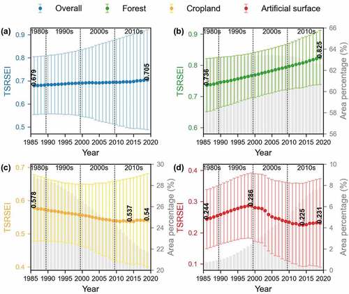
Figure 11. Relative changes of the RSEI in relation to four relevant indices (greenness, dryness, humidity, and heat) during 1986–2019. (a) Relative changes of the four indices among the main land use and cover types, measured by differences in normalized indices. Note that the increases in dryness and heat represent a negative effect for ecological quality. Three typical regions with the four intervals of 1986, 1997, 2008, and 2019 are used to represent long-term changes in normalized greenness for forest (b), normalized humidity for cropland (c), and normalized heat for artificial surfaces (d). Photos taken in 2019 of Hangzhou to illustrate (e) the global greening phenomenon for the forest ecosystem, (f) the cropland degradation phenomenon due to decreasing humidity, and (g) the urban heat island effect caused by high-density built-up areas.
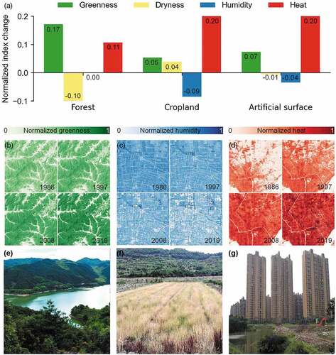
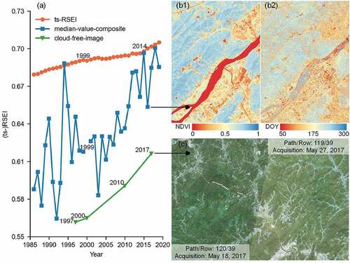
Figure 12. Comparison of methods for RSEI construction. (a) Performances of the three methods for RSEI construction based on continuous change detection (our approach), cloud-free images, and median value composition. (b1–b2) NDVI image composed of median values and its corresponding Day Of Year (DOY). (c) Mosaic image from two scenes of real Landsat images with near acquisition dates.
Supplemental Material
Download MS Word (1.5 MB)Data availability statement
All the Landsat images are freely downloaded in the LEDAPS at https://espa.cr.usgs.gov/, the Globeland30 land cover maps are freely downloaded at http://www.globallandcover.com/, and the CCDC codes used in this study are available in GitHub at https://github.com/GERSL/CCDC.