
Figures & data
Figure 1. The location of the study areas and the land-cover types of California, where wildfires were reported during the 2017 fire season in northern California (red polygon) and in Southern California (blue polygon), respectively. The land-cover map is based on the National Land Cover Database (NLCD) in 2016 (Dewitz Citation2019). The land cover is grouped into eight general types including Barren, cultivate, Developed, Forest, Herbaceous, Shrubland, Water, and Wetlands.
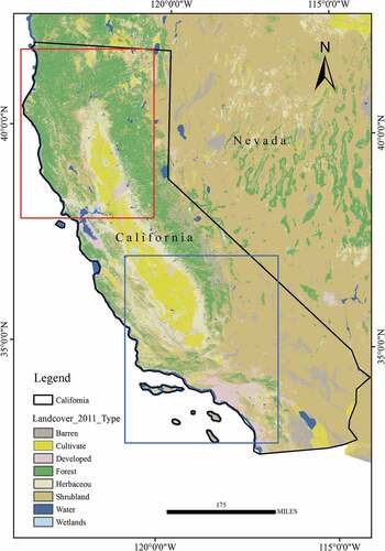
Table 1. Specifications of the medium spatial resolution sensors used for BA mapping.
Table 2. Summary of scenes used to detect BAs in California based on the spatial and temporal extensions of daily wildfire points.
Figure 2. Conceptual representation of the steps for mapping BAs in near real-time using multi-source satellite images.
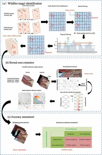
Figure 3. The spatial distribution of the training points for the “Thomas” wildfires occurred on 4 December in southern California (the Sentinel-2B image was acquired on 8 December, 2017 and is illustrated with band 8/4/3). The left panel with training points of different colors is the zoom-in area in the black rectangle of the top right panel. The training points for each class of burned area, heavy smoke2, heavy smoke1, thin smoke1, and thin smoke2 are rendered in red, green, orange, blue, and yellow colors, respectively.
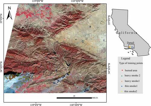
Table 3. Spectral indices used in this study (bands (B) (refer to OLI band order shown in ).
Figure 4. Spatial and temporal distribution of the detected wildfire points in (a) northern and (b) southern California. Figure (a) and (b) are the zoom-in areas in the black rectangles of the entire California in the inset maps, respectively. Wildfire points detected on the different dates from 7to31 October are rendered in different colors from dark green to red. Wildfire points that are not illustrated by the current figure (a or b) are rendered in the red color in the inset maps of the entire California illustrated on the left side of each figure.
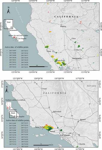
Figure 5. Boxplots of different spectral indices’ values under each scenario of the “Thomas” wildfire that occurred on 5 December based on Sentinel-2A/2B sensors. The spectral indices form roughly 3 groups and the differences within these groups are not particularly significant. The dNBR, dNIR, and NIR show great capability in distinguishing BA from other types, while dSWIR1, dSWIR2, SWIR1, and SWIR2 both exhibit great potential in discriminating HS2 from other classes. However, there is no spectral index that shows a prominent advantage in separating TS2 from other classes (1 represents samples falling outside BA, 2 represents samples falling within BA. BA, HS, and TS are the abbreviation of burned area, Heavy smoke area, and Thin smoke area, respectively).
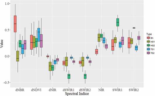
Table 4. F1-score of each set of candidate threshold values of dNBR and dSWIR for the 200 samples (100 unburned samples and 100 burned samples) for the “Thomas” wildfire occurred on 5 December based on the Sentinel-2B image.
Figure 6. The spatial distribution and monitoring time of BAs in (a) northern and (b) southern California. (a) and (b) show the detected BAs of northern and southern California wildfires, respectively. The top panels display the zoom-in BAs in black rectangles in the insets for the entire California. The bottom panels display the zoom-in BAs in the green and yellow rectangles in the insets for the entire California shown in the top right of the top panels. The detected BAs at different times are rendered in different colors from yellow to red.
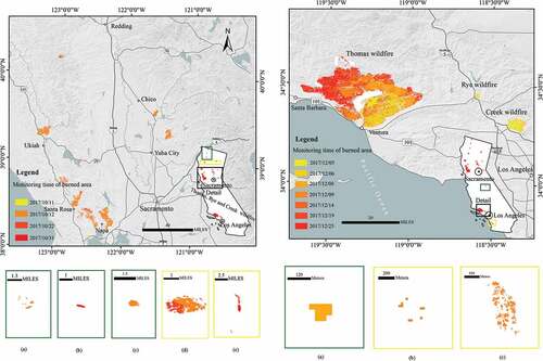
Figure 7. BA at each monitoring time in (a) northern and (b) southern California. Each bar in Figure 7 represents the BA (left axis) at each monitoring time, and the solid black line denotes the cumulative BA (right axis) at each monitoring date (solid square) as wildfires evolve.
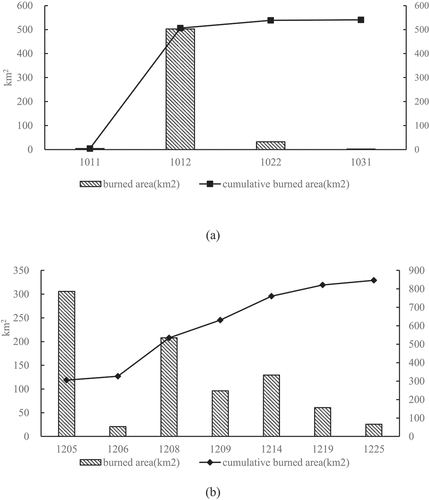
Table 5. The total BA for each vegetation type in California.
Table 6. Classification accuracy of BAs by wildfire from our automated monitoring method.