Spatiotemporal patterns of remotely sensed phenology and their response to climate change and topography in subtropical bamboo forests during 2001-2017: a case study in Zhejiang Province, China

Figures & data

Figure 1. (a) Meteorological stations, (b) bamboo abundance distribution and (c) elevation data of Zhejiang Province.

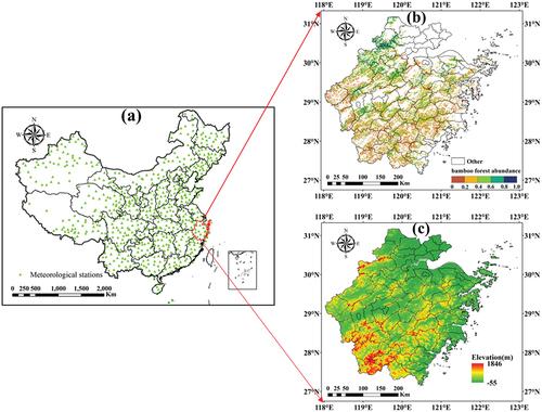
Figure 2. The flowchart of spatiotemporal patterns of bamboo forest phenology and its response to climate change and topography.

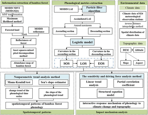
Figure 3. (a) Phenological metrics of the bamboo forest extracted based on the assimilated LAI time series, (b) comparison between the ground-observed and predicted phenological metrics using the assimilated LAI and smoothed MODIS LAI. ROC represents the curvature value of the LAI time series data fitted by the logistic regression equation. PF_Pre_SOS, PF_Pre_EOS and PF_Pre_LOS represent the predicted SOS-, EOS- and LOS-based assimilated LAI time series, respectively. MODIS_Pre_SOS, MODIS_Pre_EOS and MODIS_Pre_LOS represent the predicted SOS, EOS and LOS based on the smoothed MODIS LAI, respectively.

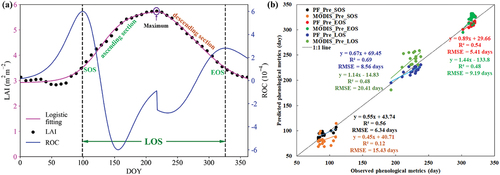
Figure 4. The spatial patterns of the average annual (a) SOS, (c) EOS, and (e) LOS and the Sen’s slope of (b) SOS, (d) EOS, and (f) LOS in Zhejiang Province.

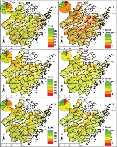
Figure 5. The change trends in the average SOS, EOS and LOS in Zhejiang Province from 2001–2017. The shadow area represents the 95% confidence intervals of the linear fitting curve of phenological annual change.

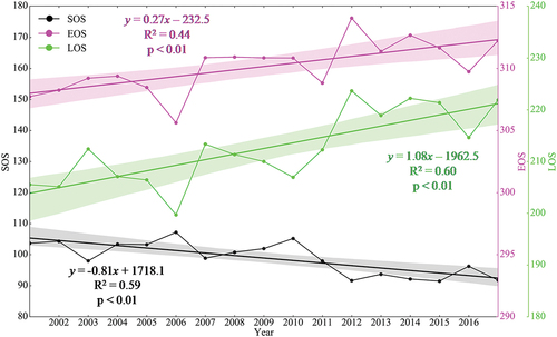
Figure 6. Spatial variations in PCCs between (a) SOS and Pre, (b) EOS and Pre, (c) LOS and Pre, (d) SOS and Rad, (e) EOS and Rad, (f) LOS and Rad, (g) SOS and Tmax, (h) EOS and Tmax, (i) LOS and Tmax, (j) SOS and Tmin, (k) EOS and Tmin, and (l) LOS and Tmin in Zhejiang Province from 2001–2017.

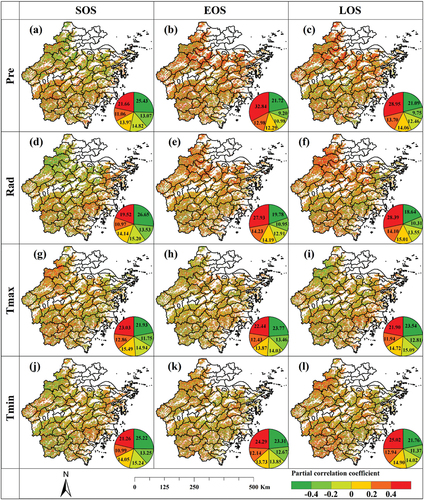
Table 1. The percentages of significant PCCs between the phenological metrics and climate variables (+ represents positive significance; - represents negative significance).

Proportion of significance		Pre	Rad	Tmax	Tmin
SOS	+	2.17%	1.75%	2.50%	2.01%
	-	3.16%	2.97%	2.00%	2.71%
EOS	+	6.23%	4.24%	2.81%	2.78%
	-	2.29%	2.05%	2.95%	2.65%
LOS	+	4.49%	3.57%	2.11%	2.68%
	-	2.18%	1.65%	2.66%	2.14%

Figure 7. Spatial sensitivity change of (a) SOS to Pre, (b) EOS to Pre, (c) SOS to Rad, (d) EOS to Rad, (e) SOS to Tmax, (f) EOS to Tmax, (g) SOS to Tmin, and (h) EOS to Tmin in Zhejiang Province.

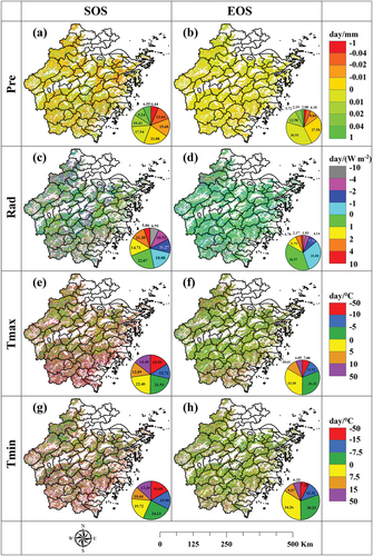
Figure 8. Path analysis of the influence of meteorological factors on phenological metrics based on the path model.

*** represents p<0.01.

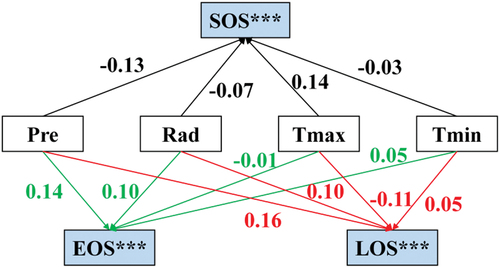
Figure 9. Change trends in (a) SOS, (b) EOS, and (c) LOS with altitude, (d) SOS, (e) EOS, (f) LOS with slope, (g) SOS, (h) EOS, and (i) LOS with aspect in Zhejiang Province. The shadow area of (a)-(f) represents the 95% confidence interval (CI) of the fitting curve.

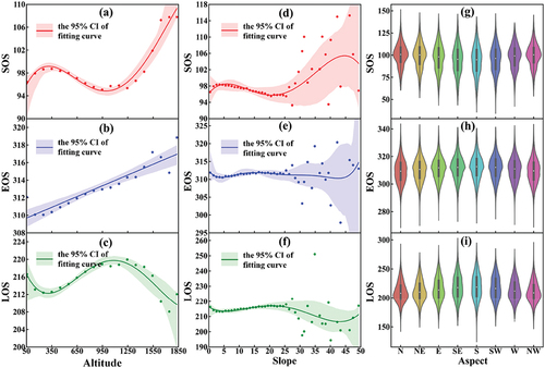
Figure 10. The PCCs between phenology and climatic factors along with (a) altitude, (b) slope and (c) aspect in Zhejiang Province.

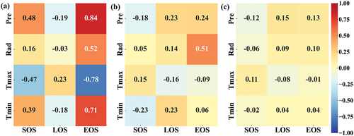
Figure 11. Analysis of influences on phenological driving factors based on the PLS-PM model. Circles represent the LVs. Rectangles represent the MVs. Arrows represent the links between MVs and associated LVs, as well as among related LVs, while arrow labels are the correlation coefficients and PCs that quantify those links. Solid arrows and dashed arrows indicate direct and indirect impacts, respectively.

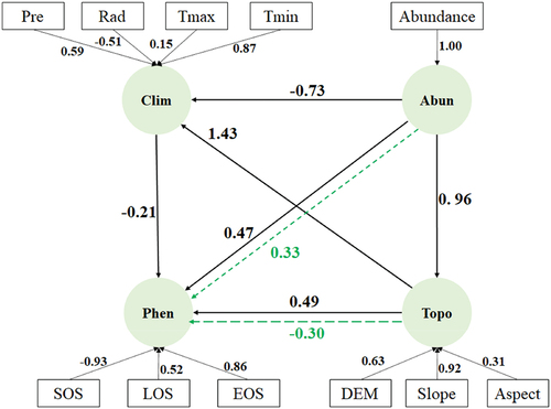
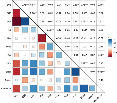
Figure 12. The correlation coefficient between phenological factors and driving factors based on the Pearson correlation coefficient method.

*, ** and *** represent p<0.1, p<0.05 and p<0.01, respectively.

Data availability statement

The MODIS, Climate and DEM datasets used during this study are openly available from NASA’s website (https://ladsweb.modaps.eosdis.nasa.gov/search/), the National Meteorological Science Data Center of China (http://data.cma.cn/), and the Geospatial Data Cloud site, the Computer Network Information Center, and the Chinese Academy of Sciences (http://www.gscloud.cn), respectively.