
Figures & data
Figure 1. The architecture of multi-scale features extraction network (MSFENet), including four residual blocks (RB) which are composed of several basic blocks (BB), four dense atrous convolution modules (DACM), and five decoder blocks (DB).
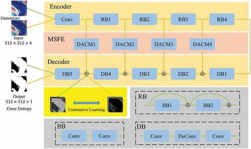
Figure 2. Atrous convolution kernels with dilation rate of 1 (a), 3 (b) and 5 (c).
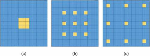
Figure 3. The structure of dense atrous convolution module (DACM).
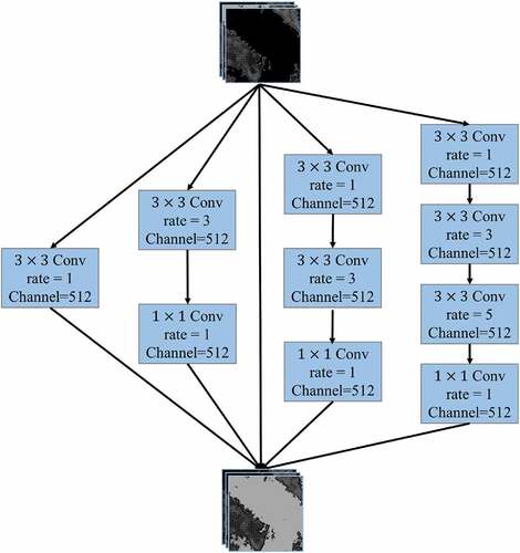
Figure 4. Illustration of pixel-level positive and negative sample pairs. Different colours represent different categories. Ac, Ad, Ba, Bb, Cc, Cd, Dc, and Dd are positive sample pairs. Aa, Ab, Bc, Bd, Ca, Cb, Da, and Db are negative sample pairs.
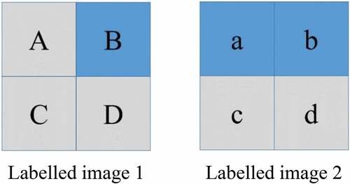
Figure 5. Four selected GF-2 images and the corresponding labelled images. Row a shows standard false color of GF-2 images, Row B shows labelled images in LSCS, and Row C shows relabelled images by visual interpretation.
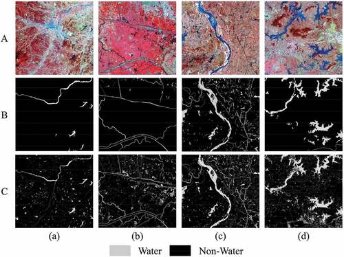
Figure 6. Two regions mainly containing small water bodies, (a), (b), and (c) are GF-2 image, labelled image in LSCS, and relabelled image, respectively.
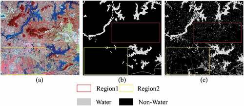
Figure 7. The water area distribution histogram of region 1 (a), region 2 (b), and cumulative water area distribution histogram of region 1 (c), region 2 (d).
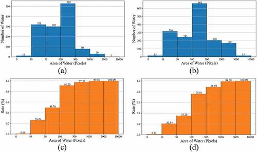
Table 1. Accuracy assessment results of water label image in LSCS.
Figure 8. Water bodies prediction process using deep learning models. The yellow boxes represent valid areas after cropping, and the red boxes represent all areas after cropping.
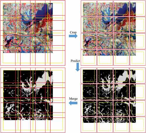
Table 2. Accuracy assessment results of ablation study on test set (bold numbers refer to the highest values).
Table 3. Accuracy assessment results of ablation study on region 1 (bold numbers refer to the highest values).
Table 4. Accuracy assessment results of ablation study on region 2 (bold numbers refer to the highest values).
Figure 9. Water extraction results with different network configurations. (a) Image, (b) Ground truth, (c) the Baseline, (d) the Baseline + SC, (e) the MSFENet, and (f) the MSFENet + CL.
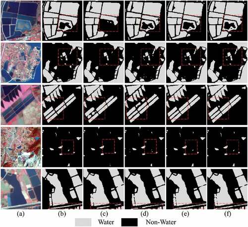
Figure 10. Accuracy curves with the increasing of sample sizes. (a) test set, (b) region 1, and (c) region 2.
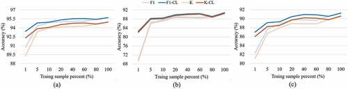
Table 5. Accuracy assessment results when 1% of the training samples are used (bold numbers refer to the highest values).
Table 6. Accuracy assessment results of different methods on test set (bold numbers refer to the highest values).
Figure 11. Water extraction results with different methods. (a) Image, (b) Ground truth, (c) NDWI, (d) RF, (e) FCN, (f) PSPNet, (g) UNet, (h) DeepLabv3+, and (i) MSFENet.
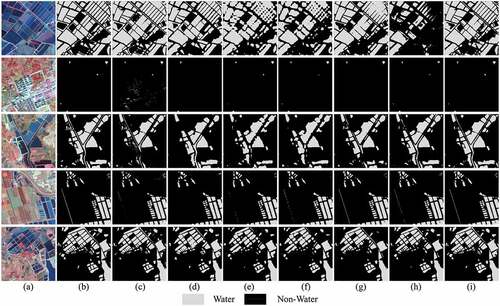
Table 7. Accuracy assessment results with different methods in region 1 (bold numbers refer to the highest values).
Table 8. Accuracy assessment results with different methods in region 2 (bold numbers refer to the highest values).
Figure 12. The GF-2 image in the test set (a) and simulated image (b).
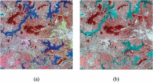
Figure 13. Water extraction results of different methods on the simulated image. (a) Image, (b) Ground truth, (c) FCN, (d) PSPNet, (e) UNet, (f) DeepLabv3+ and (g) MSFENet.
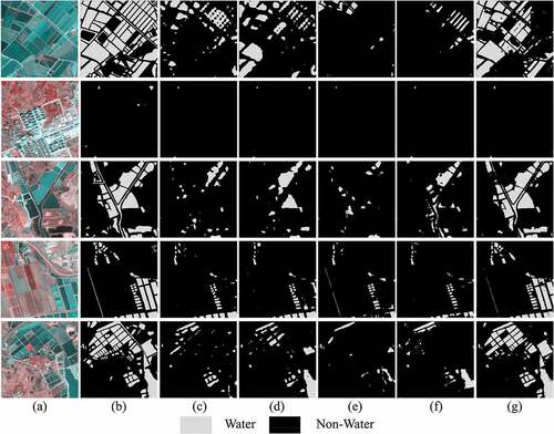
Table 9. Accuracy assessment results of different methods on the simulated image (bold numbers refer to the highest values).
Table 10. Accuracy assessment results of different methods on the region 1 of the simulated image (bold numbers refer to the highest values).
Table 11. Accuracy assessment results of different methods on the region 1 of the simulated image (bold numbers refer to the highest values).
Figure 14. Water extraction results of different methods in LoveDA. (a) Image, (b) Ground truth, (c) FCN, (d) PSPNet, (e) UNet, (f) DeepLabv3+, and (g) MSFENet.
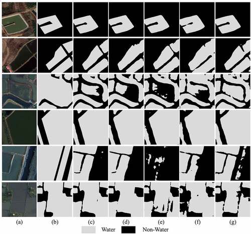
Table 12. Accuracy assessment results of different methods in LoveDA (bold numbers refer to the highest values).
Data availability statement
The GF-2 images are freely available as follows, Gaofen Image Dataset (GID): https://x-ytong.github.io/project/GID.html. The LoveDA are freely available as follows: https://github.com/Junjue-Wang/LoveDA And the relabeled images and codes that support the findings of this study are available from the corresponding author, upon reasonable request.