Revealing the time lag between slope stability and reservoir water fluctuation from InSAR observations and wavelet tools— a case study in Maoergai Reservoir (China)

Figures & data

Figure 1. (a) Overview of the study area; and (b) the reservoir area.

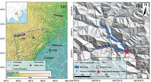
Figure 2. Spatial and temporal baseline diagrams of interferograms obtained from (a) ascending; and (b) descending images.

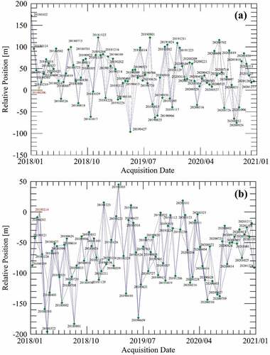
Figure 3. Proposed flow chart for the analysis of InSAR time series of the unstable slopes of Maoergai Reservoir.

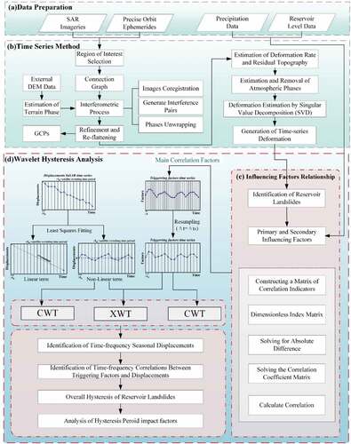
Figure 4. (a) SBAS-InSAR displacement rate results of the Maoergai reservoir in ascending orbiting; (b)sbas-InSAR displacement rate results of the Maoergai reservoir in descending orbiting; (c) Geometric distortion of the ascending orbiting; (d) Geometric distortion of the descending orbiting.

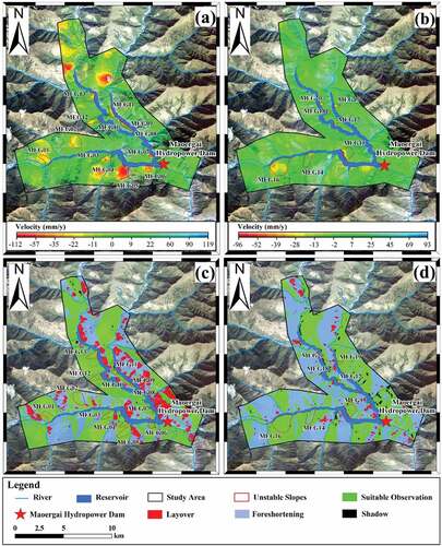
Figure 5. Average displacement rate of unstable slopes (MEG01–13 detected in the ascending data and MEG14–20 detected in the descending data).

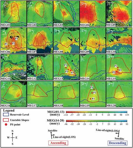
Figure 6. Time series displacement curves of landslides (a) MEG06; (b) MEG13; (c) MEG15; and (d) MEG19.

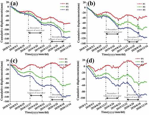
Figure 7. Yearly relationship between cumulative displacements and influence factors.

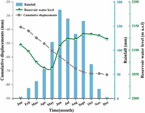
Figure 8. Correlation between cumulative displacements and influencing factors derived from gray correlation analysis.

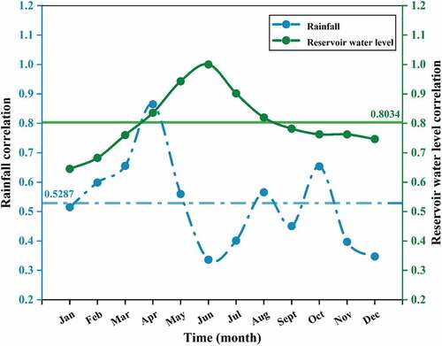
Figure 9. (a) Reservoir water level time series after resampling; (b) CWT of MEG02; (c) CWT of MEG09; (d) CWT of MEG13; (e) CWT of MEG15; (f) CWT of MEG18. 5% significance level relative to red noise is shown as a coarse contour. The wavelets are not fully localized in time and there may be edge pseudo-effects out of the cone of influence (COI).

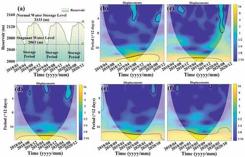
Figure 10. Results from cross-wavelet transform (XWT) for the reservoir non-linear displacements with reservoir water level. The black line separates ascending orbiting results (above) from descending orbiting results (below). 5% significance level relative to red noise is shown as a coarse contour. The wavelets are not fully localized in time and there may be edge pseudo-effects out of the cone of influence (COI).

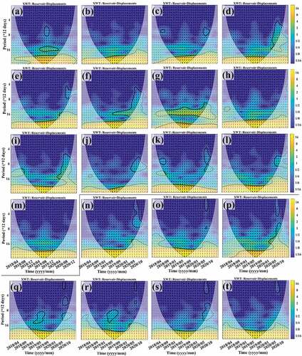
Figure 11. (A) Interannual cycle time lag distribution; (b) time lag and influence factors correlation. The grey dotted lines correspond to the fitted line of each scattered point.

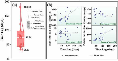
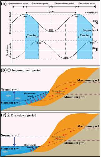
Figure 12. Conceptual interpretation of the non-linear displacements. a) Time series relationship; b) Impoundment period; c) Drawdown period.

Data availability statement

All relevant data are available from the authors upon reasonable request. Some datasets that support the findings of this study are available in [https://scihub.copernicus.eu/dhus/#/home], [https://earthexplorer.usgs.gov/], [https://disc.gsfc.nasa.gov/].