Exact Voronoi diagram for topographic spatial analysis

Figures & data

Figure 1. A surface grid and a standard Laplacian discretization of the PDE methods. The Laplace-cotan operator is formulated as ${\left(Lu\right)}_i=\frac{1}{2A_i}\sum _j\left(cot{\alpha }_{ij}+cot{\alpha }_{ji}\right)\left(u_j-u_i\right)$, where $u_i$ is the heat value at vertex $x_i$,$A_i$ is the one-third area of the triangles incident to vertex $x_i$, from Bobenko and Springborn (2007). Notably, whatever how delicate the operators are, they are approximations of the continuous heat derivatives in time and space, whereas the underlying Earth surface is rather rough than smooth.

Figure 2. Computational geometry methods organize the geodesic wave propagation in linearly truncated windows. five windows (i.e. waves) emanated from the source S in the first propagation. The wave $\stackrel{\hspace{0.17em}}{BA}$ was back-pruned as $\stackrel{\hspace{0.17em}}{B{n}_1}$ and $\stackrel{\hspace{0.17em}}{n_{1}A}$ in the following propagation. vertex B was an obstacle point where the wave was bifurcated into three parts. For the invisible to source part of $\stackrel{\hspace{0.17em}}{s_0{s}_1}$,the propagation was not stopped but relayed by vertex B. The dotted lines show a portion of the implicit splitting. The red-to-blue color indicates the distance increase.

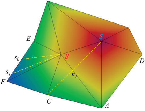
Figure 3. Excess a prior mesh splitting (the grids in red) for approximating the geodesic (the solid curve in blue) of graph-based methods, from Kanai and Suzuki (2001). Because there is no exact information for reference, the geodesic is searched and approximated from the excess paths. More delicate pre-computations for graph-based geodesics are referred to Ying, Wang, and He (2013) and Xin et al. (2018).

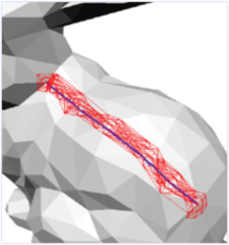
Figure 4. TIN grid M definition in planar space. The point list V defines the geometry, the facet list F defines the topology with indices to V (the edge list E is usually implicit). The combinatorial topology stresses the regularity that each k-cell’s boundary is constrained by the (k-1)-cells. this regularity is strictly required by the MMP/VTP algorithms for propagation convenience, while other algorithms such as the heat method (Sharp et al. 2019) may only requires a loose topology as point clouds. The sources are surface points, meaning that they are not confined to mesh vertices or mesh edges (see Fig 11, right).

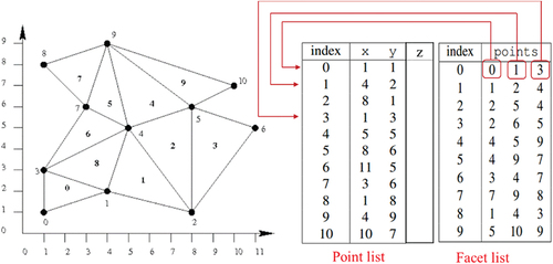
Figure 5. A topographic bump bifurcates the geodesic wavefront. A saddle point sites at vertex A and a source sites at the surface point P (left). right, the unfolding all facets adjacent to saddle A onto the AEF plane causes source P has two images. $\mathrm{\angle }{I}_{1}A{I}_2$ denotes the angle defect. The wavefront from source P is bifurcated at saddle A into left and right parts and the relayed part. note that the relayed part has a smaller radius, which indicates the differentiated propagation velocity.

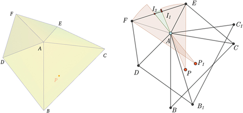
Figure 6. Circular wavefronts meet and spatial competition is equilibrated as singular loci. left: wavefronts from different sources P₀ and P₁ meet at singularity S₀₀; right: wavefronts from different directions of the same pseudo-sources P₁/P₂ meet at singularity S₀₁. At a meeting point, a hyperbola can be grown (see light-green dotted curve) for space equilibration on behalf of its left/right windows. note the solid-green directional arcs are truncated by the facet for further use.

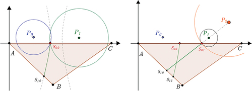
Figure 7. Steep terrain (rendered in height) with six sources (white points) and the trimmed bisectors (green arcs). A close view of the hyperbolic arc $\stackrel{\hspace{0.17em}}{MN}$ is drawn on the right and compared to the line segment (white), where M/N are break points, and vertex A (the red point) is the saddle. The terrain data is a fragment of the SRTM DEM (90 m resolution) in the Himalaya mountain region and can be found in the supplementary material.

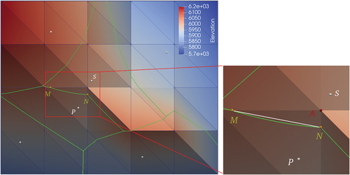
Figure 8. Singular grow of the visibility windows from six distinct sources P0–P5. (a) Conic tessellation of singular loci in the first round of growth, where I0–I2 are the three candidate intersections for the new singularities. (b) two new singularities determined at the effective near intersections, with the growth of windows S10AS00 and S01BS21 being satisfied. (c) New singular loci grown from the new singularities. (d) growth of windows S11S10 and S21S20 satisfied. (e) final space equilibrium of the six sources on the boundary facet.

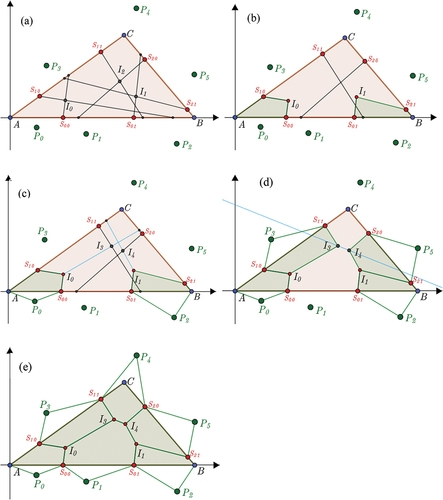
Figure 9. Stages of the GVD algorithm. From left to right: non-boundary facet clustering, boundary facet tessellation, and re-clustering of the tessellated sub-facets and the GVD structure extraction.

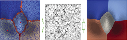
Figure 10. Experimental topographic TIN grid rendered in elevation (left). it is located in the region of Mount Saint Helens, near Spirit Lake, Washington, US (right).

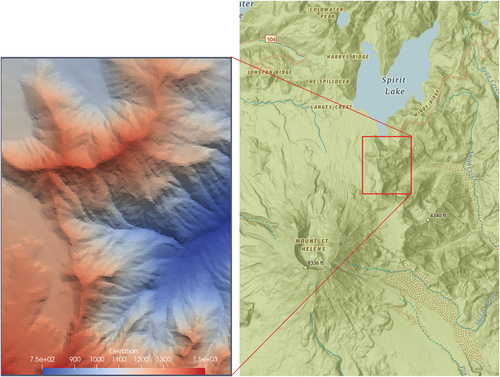
Figure 11. GVD (green curves) with 30 random sources (yellow points), with a close view on the right.

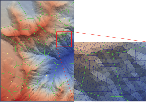
Figure 12. GVD dual TINs compared with the D2D TINs. (a) GVD dual TIN (green) with 30 random sources. (b) D2D TIN (blue) overlaid with the GVD TIN to expose the inconsistent green edges where D2D is potentially incorrect. overlaid TINs for (c) 50 and (d) 100 random sources, with the green edges showing the inconsistencies. The base map consists of the GVD cells rendered with distinct colors.

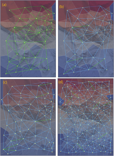
Table 1. Maximized minimal angles (°) in the inconsistent triangles between the GVD TIN and the D2D TIN.

GROUP	1	2	3	4	5	6	7
GVD	42.03	34.96	39.01	38.11	34.66	41.15	37.78
	44.79	52.33	44.05	45.31	35.53	41.57	52.85
D2D	41.12	30.62	33.11	34.69	34.60	37.33	36.97
	43.88	38.39	42.96	43.99	40.69	47.05	39.71

Table 2. Areas (m²) and shrunk rate (%) of the inconsistencies in the GVD dual TIN and D2D TIN, referenced to the ground truth areas.

Sample Resolution		30	50	100
GVD	area (m^2)	1,128,693.49	717,703.38	1,705,398.05
	shrunk rate (%)	8.84	5.09	6.94
D2D	area (m^2)	1,123,050.19	716,130.21	1,696,663.45
	shrunk rate (%)	9.30	5.30	7.42
Ground Truth (m^2)		1,238,179.07	756,200.58	1,832,634.64

Figure 13. Step-wise subdivision of the boundary facets of TIN mesh in Figure 7. GVD edge arcs are drawn in green for reference. In (a)/(b), the facet highlighted in purple contains 4 singularities and need to be subdivided. (c) shows the final subdivision with no facet containing 4 or more sources.

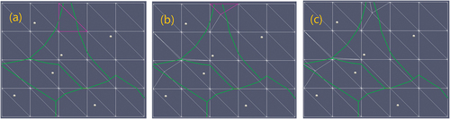
Figure 14. Initial states and final states of the exact GVD (a/d), rGvd(b/e), and lGVD (c/f) on CVT optimizations. The same 100 random points are used as the sources. The exact GVD sources and cells are in yellow and green, the rGVD sources and cells are in blue, and the lGVD sources and cells are in white.

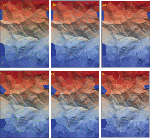
Figure 15. Overlaid final states of the exact GVD and rGVD (a), exact GVD and lGVD (b). The sources and cells of the exact GVD are in yellow and green, the sources and cells of rGVD are in blue, and the sources and cells of lGVD are in white.

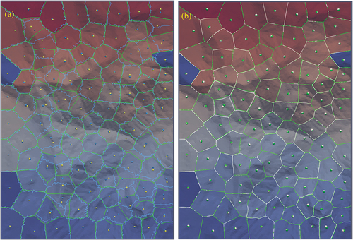
Figure 16. Trajectories of the GVD (green) diffusion centroids compared with those of rGVD (blue) and lGVD (white). The trajectories of the centroids are sparse at the initial stage and dense at the final stage. (a) comparison of GVD and rGVD. (b) Oppposite optimization directions of rGVD and GVD. (c) early convergence of rGVD than of GVD. (d) comparison of GVD and lGVD. (e) Biased and early stopped optimization of lGVD.

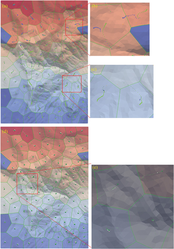
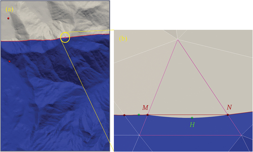
Figure 17. Bisector exactness at macro scale and facet scale. (a) hardly discernible difference between the lGVD bisector (red curve) and the exact GVD boundary, with a facet circled in bright yellow for checking. (b) prominent difference found at the facet scale, where a linear scheme directly connected break points on the edge (M/N) for approximation and missed the characteristic edge shape for ignoring the break point (H) inside the facet.

Bobenko, A. I., and B. A. Springborn. 2007. “A Discrete Laplace–Beltrami Operator for Simplicial Surfaces.” Discrete & Computational Geometry 38 (4): 740–756. doi:10.1007/s00454-007-9006-1.

 Web of Science ®Google Scholar

Kanai, T., and H. Suzuki. 2001. “Approximate Shortest Path on a Polyhedral Surface and Its Applications.” Computer-Aided Design 33 (11): 801–811. doi:10.1016/S0010-4485(01)00097-5.

 Web of Science ®Google Scholar

Ying, X., X. Wang, and Y. He. 2013. “Saddle Vertex Graph (SVG): A Novel Solution to the Discrete Geodesic Problem.” ACM Transactions on Graphics 32 (6): 1–12. doi:10.1145/2508363.2508379.

 Web of Science ®Google Scholar

Xin, S., W. Wang, Y. He, Y. Zhou, S. Chen, C. Tu, and Z. Shu. 2018. “Lightweight Preprocessing and Fast Query of Geodesic Distance via Proximity Graph.” Computer-Aided Design 102: 128–138. doi:10.1016/j.cad.2018.04.021.

 Web of Science ®Google Scholar

Sharp, N., Y. Soliman, and K. Crane. 2019. “The Vector Heat Method.” ACM transactions on graphics 38 (3): 24.21–24.19. doi:10.1145/3243651

 Web of Science ®Google Scholar

Data availability statement

The data that support the findings of this study are available in GitHub at: https://github.com/sanchopanza72/gvd_topographic