Spatially continuous mapping of hourly ground ozone levels assisted by Himawari-8 short wave radiation products

Figures & data

Figure 1. Spatial distribution of the discrete O₃ monitoring network conducted by the China National Environmental Monitoring Center (CNMEC). (Elevation was derived from consortium for spatial information of the US geological survey).

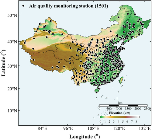
Table 1. Collection of datasets used in this study.

Data	Variable	Unit	Temporal resolution	Spatial resolution	Source
O3	O3	µg/m^3	1 h	site	CNEMC
SWR factors	UVA	W/m^2	1 h	5km	Himawari-8
	UVB	W/m^2	1 h	5km
	SWR	W/m^2	1 h	5km
Atmospheric scattering factors	AOD	Unitless	1 h	~0.375°
	PM10	µg/m^3	1 h	~0.375°
Background O3	CO	mol/cm^2	daily	1°	MOPITT
	SCO	DU	daily	165 km x 3 km	MLS
	TCO	DU	daily	0.25°	OMI
Ozone precursor	NO2	molec/cm^2	daily	0.25°
	HCHO	molec/cm^2	daily	0.25°
Meteorological factor	TEMP	K	1 h	0.1°	ERA5
	WS	m/s	1 h	0.1°
	ET	mm	1 h	0.1°
	PRES	hpa	1 h	0.1°
	BLH	m	1 h	0.25°
	RH	%	1 h	0.25°
	STRD	J/m^2	1 h	0.25°
Land type factor	NDVI	Unitless	16 days	0.05°	MODIS
	LUC	Unitless	year	0.05°
Topographic factor	DEM	m	-	90m	USGS

Figure 2. Scatterplot of estimated ground-level ozone concentrations from the conducted model versus corresponding site-based observations for (a) 20 clusters based on spatial K-means method, (b)all available samples, (c)20-fold cluster-based CV, (d)10-fold site-based CV, (e)10-fold sample-based CV. The RMSE, MAE, rRMSE, number of samplings (N), R² and the linear-regression function are displayed in each scatterplot.

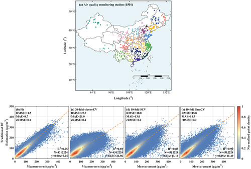
Figure 3. Scatterplot of seasonal estimated ground-level ozone concentrations from conducted model versus corresponding site-based observations for (a-d) direct fitting of available data for each season, (e-h) 20-fold cluster-based seasonal CV, (i-l) 10-fold site-based seasonal CV, and (m-p) 10-fold sample-based seasonal CV. The RMSE, MAE, rRMSE, number of samplings (N), R² and the linear-regression function are displayed in each subplot.

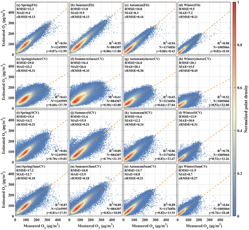
Figure 4. Scatterplot of diurnal estimated ground-level ozone concentrations from conducted model versus corresponding site-based observations for (a-h) 20-fold cluster-based CV for each diurnal time periods, (i-p)10-fold sample-based diurnal CV, (q-x) 10-fold site-based seasonal CV. The RMSE, MAE, rRMSE, number of samplings (N), R² and the linear-regression function are displayed in each subplot.

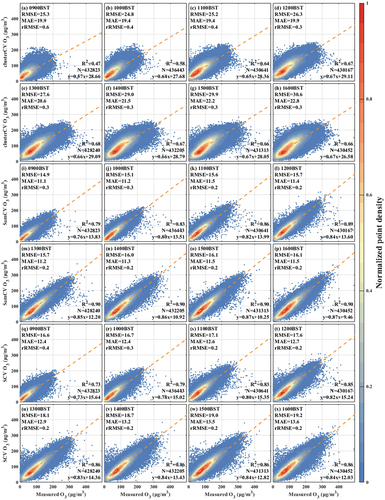
Figure 5. Variation of (a) daily averaged estimated O₃ concentrations versus measured O₃ and (b) daily averaged estimation bias.

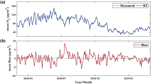
Figure 6. Spatial distribution of estimated performance from conducted model versus corresponding site-based observations for sample number (a), R² (b), MAE (c), RMSE (d).

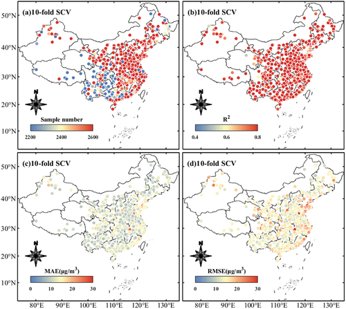
Figure 7. Spatial distribution of estimated performance from conducted model versus corresponding cluster-based observations for sample number (a), R² (b), MAE (c), RMSE (d).

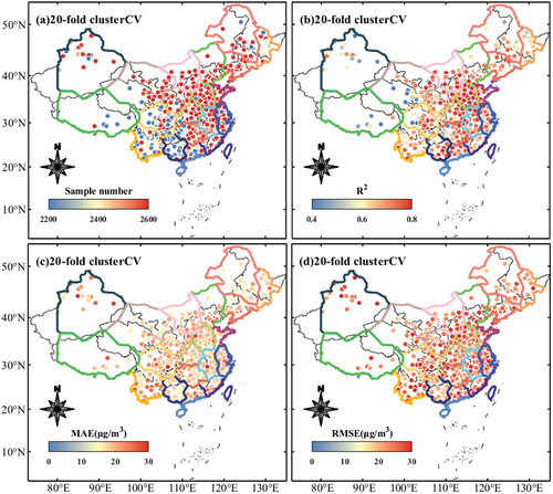
Figure 8. Spatial distribution of seasonal average estimated ozone concentration.

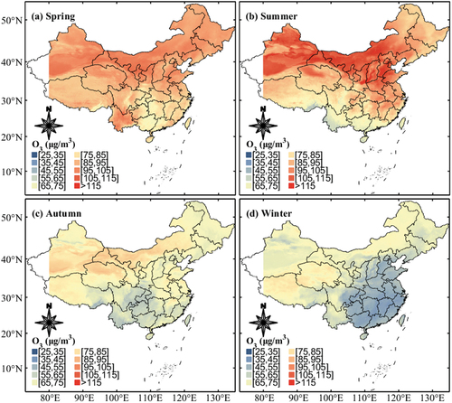
Figure 9. Verification of spatial distribution of seasonal average O₃. The site-based seasonal mean ground-level ozone concentrations are represented by tinctorial circles.

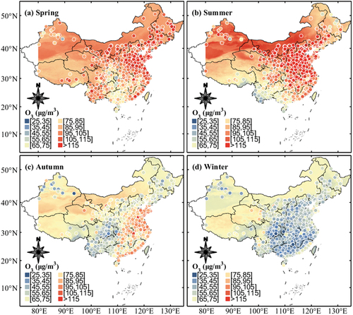
Figure 10. Spatial distribution of average estimated ground-level ozone concentrations for (a) all available data, and (b-i) different diurnal hours (0900 BST-1600 BST).

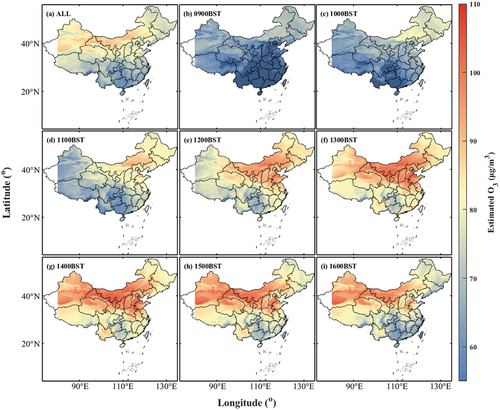
Figure 11. Verification of spatial distribution of hourly average O₃. The site-based hourly mean ground-level ozone concentrations are represented by tinctorial circles.

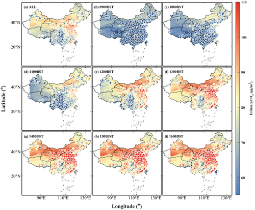
Figure 12. Spatial distribution of hourly estimated ozone concentration on a specific day (Take June 30th, 2018 as an example, and the Beijing-Tianjin-Hebei is displayed as a typical region with severe surface ozone pollution. The top picture shows the whole country, and the bottom picture shows the Beijing-Tianjin-Hebei region).

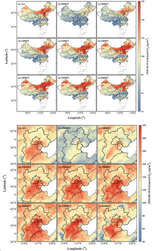
Figure 13. Verification of spatial distribution of hourly estimated ozone concentration on a specific day (The top picture shows the whole country, and the bottom picture shows the Beijing-Tianjin-Hebei region). The site-based hourly mean ground-level ozone concentrations at corresponding date are represented by tinctorial circles (Take June 30th, 2018 as an example, and the Beijing-Tianjin-Hebei is displayed as a typical region with severe surface ozone pollution).

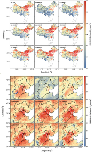
Figure 14. distribution of averaged estimated ground-level ozone concentration for (a)weekdays, (b)weekends, (c)differential between weekdays and weekends and (d)salient region under different ozone generation mechanisms.

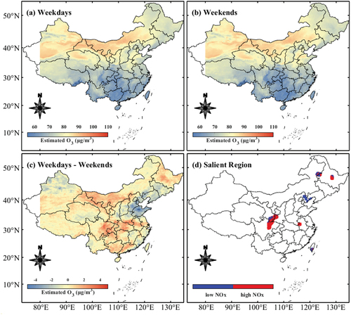
Table 2. Comparison of previous O₃ studies focused on China.

Model	Respond	TR	SR	Validation			Study period	Spatial continuity	Literature
				R^2	MAE	RMSE
XGBoost	MDA8	Daily	0.1°×0.1°	0.64	21.47	-	2013–2017	NO	(Liu et al. 2020)
Data fusion	MDA8	Daily	0.1°×0.1°	0.70	26.20	16.70	2013–2017	YES	(Xue et al. 2020)
GWR	MAO3	Monthly	0.25°×0.25°	0.77	8.14	-	2014	YES	(Zhang et al. 2020)
RF, LightGBM	MDA8	Daily	0.25°×0.25°	0.79	-	17.09	2018	YES	(Song, Li et al. 2022)
STET	MDA8	Daily	0.1°×0.1°	0.80	13.87	21.10	2013–2020	YES	(Wei, Li et al. 2022)
SGLboost	O3	Hourly	2km	0.85	-	19.04	2017–2019	NO	(Wang et al. 2022)
BT	O3	Hourly	5km	0.87	13.30	18.30	2018–2019	YES	This study

XGBoost: eXtreme Gradient Boosting; GWR: geographically weighted regression; RF: random forest; STET: space-time extremely randomized trees; LightGBM: Light Gradient Boosting; SGLboost: Self-adaptive geospatially Local scheme based on Categorical boosting; BT: bagged-tree; MDA8: maximum 8-h average ground-level O₃; MAO₃: monthly average ground-level O₃; TR: temporal resolution; SR: spatial resolution; SCV: site-based cross validation.

Figure 15. (a)Monthly *R values of estimated models with or without Himawari-8 SWR dataset. (b)The importance score of features included in BT model.

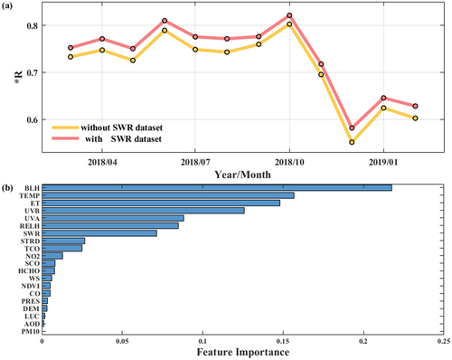
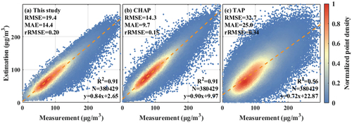
Figure 16. Comparison among this study, CHAP and TAP on the estimated performance of MDA8.

Liu, R., Z. Ma, Y. Liu, Y. Shao, W. Zhao, and J. Bi. 2020. “Spatiotemporal Distributions of Surface Ozone Levels in China from 2005 to 2017: A Machine Learning Approach.” Environment International 142: 105823. doi:10.1016/j.envint.2020.105823.

 PubMed Web of Science ®Google Scholar

Xue, T., Y. Zheng, G. Geng, Q. Xiao, X. Meng, M. Wang, X. Li, N. Wu, Q. Zhang, and T. Zhu. 2020. “Estimating Spatiotemporal Variation in Ambient Ozone Exposure During 2013–2017 Using a Data-Fusion Model.” Environmental Science & Technology 54 (23): 14877–14888. doi:10.1021/acs.est.0c03098.

 PubMed Web of Science ®Google Scholar

Zhang, X. Y., L. M. Zhao, M. M. Cheng, and D. M. Chen. 2020. “Estimating Ground-Level Ozone Concentrations in Eastern China Using Satellite-Based Precursors.” IEEE Transactions on Geoscience and Remote Sensing 99: 1–10. doi:10.1109/TGRS.2020.3038405.

 Google Scholar

Song, G., S. Li, J. Xing, J. Yang, L. Dong, H. Lin, M. Teng, S. Hu, Y. Qin, and X. Zeng. 2022. “Surface UV-Assisted Retrieval of Spatially Continuous Surface Ozone with High Spatial Transferability.” Remote Sensing of Environment 274: 112996. doi:10.1016/j.rse.2022.112996.

 Web of Science ®Google Scholar

Li, M., Q. Yang, Q. Yuan, and L. Zhu. 2022. “Estimation of High Spatial Resolution Ground-Level Ozone Concentrations Based on Landsat 8 TIR Bands with Deep Forest Model.” Chemosphere 301: 134817. doi:10.1016/j.chemosphere.2022.134817.

 PubMed Web of Science ®Google Scholar

Wang, Y., Q. Yuan, L. Zhu, and L. Zhang. 2022. “Spatiotemporal Estimation of Hourly 2-Km Ground-Level Ozone Over China Based on Himawari-8 Using a Self-Adaptive Geospatially Local Model.” Geoscience Frontiers 13 (1): 101286. doi:10.1016/j.gsf.2021.101286.

 Web of Science ®Google Scholar

Data availability statement

The raw data used in this study are publicly available from the sources provided in following links. The processed data generated from this study are available upon request to the corresponding author.

- Surface O₃ in situ data: http://www.cnemc.cn/

- Short Wave Radiation L3 data and Aerosol Property L4 data: https://www.eorc.jaxa.jp/ptree/

- MOP03J_8 L3 data: https://asdc.larc.nasa.gov/project/MOPITT/

- ML2O3_005 L2 data, OMTO3E L3 data, OMI_MINDS_NO2d L3 data, OMHCHOG L2 data, Land Cover Type (MCD12Q1) L3 data and MOD13C1/MYD13C1 L3 data: https://www.earthdata.nasa.gov/

- ERA5 reanalysis data:https://cds.climate.copernicus.eu/cdsapp#!/

- SRTM 90m DEM Digital Elevation: https://srtm.csi.cgiar.org/