
Figures & data
Figure 1. Visibility of stone walls with different imagery sources. a: Landsat 8 OLI (30 m), 3 January 2016; b: Sentinel-2 (10 m), 18 February 2016; c: Aerial photography (0.1m), March 2016; d: LiDAR derived hillshade (1m, Azimuth 315°), e: LiDAR derived slope (1m); f: Stone walls in field (yellow refers to overall physical properties of stone walls (Johnson and Ouimet Citation2016)).
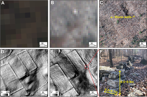
Figure 2. Study sites of this study with five training sites (including validation sites) and three test sites in Connecticut, USA. Training sites consist of (1) dense forested landscape in Ashford and (2) moderate to dense forested landscape and farmland in Woodstock, and (3) developed urban and suburban areas in Windham. Note that validation data is derived from training sites (See details about validation data in section 3.1.2). Test sites are (1) UConn forest (UF), (2) Wormwood Hill (WH) in Mansfield town, and (3) Cornwall town.
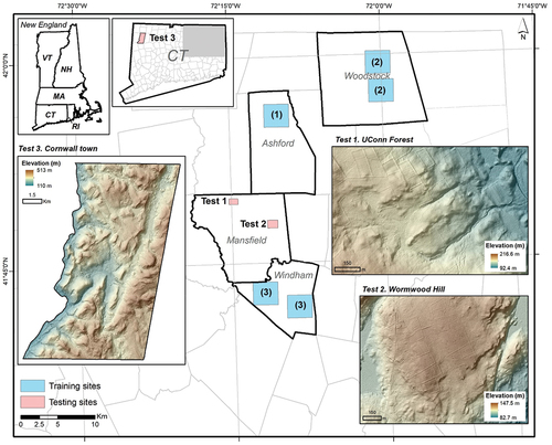
Table 1. List of collected data.
Figure 3. Workflow for the stone wall detection. Abbreviation: TP (true positives), FP (false positives), FN (false negatives), TN (true negatives).
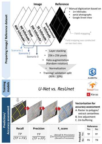
Table 2. Specific information of three input scenarios used in this study.
Figure 4. Model architectures used in this study (A: U-Net, B: ResUNet).
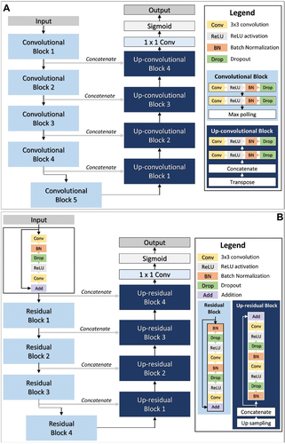
Table 3. Summary of model architecture for both U-Net and ResUNet.
Table 4. Hyperparameters for model training.
Figure 5. Vectorization process of model prediction result to minimize a potential error in accuracy assessment. A: example of errors occurred in raster-based accuracy assessment result. B: predicted stone walls (SW) by model (yellow pixel) and its centerline (black line); C: reference stone wall after line adjustment (pink line) based on extracted centerline from model (black line); D: Accuracy assessment result after vectorization process. Note that TN is true negative, TP is true positive, FN is false negative, and FP is false positive.
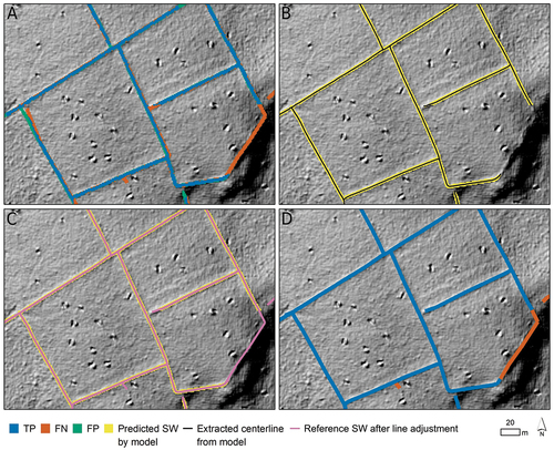
Figure 6. Workflow of post-processing (PP) for accuracy assessment in town-level model prediction result. (a: NW hillshade map; b: Manually digitized stone wall (SW) and SW predicted by U-Net S3 model overlaying three types of impervious cover (IC) in 2012 and buffered all impervious cover (Data source: CT CLEAR (Citation2017)); c: Precision example after impervious cover post-processing (IC PP); d: Recall example after impervious cover post-processing (IC PP); e: leaf-off aerial photography in 2016 (CRCoG Citation2016a); f: Manually digitized stone wall (SW) and SW predicted by U-Net S3 model overlaying land cover (LC) of 2015; G: Precision example after impervious and land cover post-processing (IC LC PP); h: Recall example after impervious and land cover post-processing (IC LC PP)).
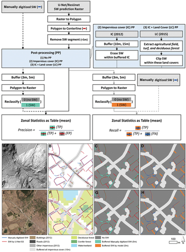
Figure 7. Binary cross entropy loss curve per epoch for U-Net/ResUnet models and three scenarios (S1, S2, and S3). (A: U-Net S1, B: U-Net S2, C: U-Net S3, D: ResUnet S1, E: ResUnet S2, F ResUnet S3).
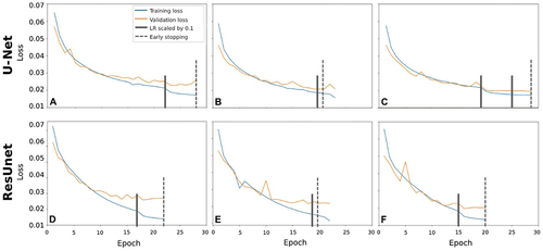
Table 5. Result of model performance with different models and scenarios.
Figure 8. The distribution of TP, FN, FP, and TN results from different models and scenarios at test site 1 (UF). a: high-resolution orthophotography (CT ECO Citation2019); A: U-Net S1; B: U-Net S2; C: U-Net S3; D: ResUnet S1; E: ResUnet S2; F: ResUnet S3. NW hillshade map is a background. Note that TN symbol is transparent to visualize background hillshades.
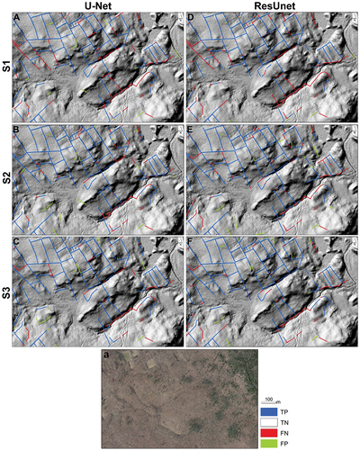
Figure 9. The distribution of TP, TN, FN, and FP results from different models and scenarios at test site 2 (WH). a: high-resolution orthophotography (CT ECO, 2019); A: U-Net S1; B: U-Net S2; C: U-Net S3; D: ResUnet S1; E: ResUnet S2; F: ResUnet S3. Note that TN symbol is transparent.
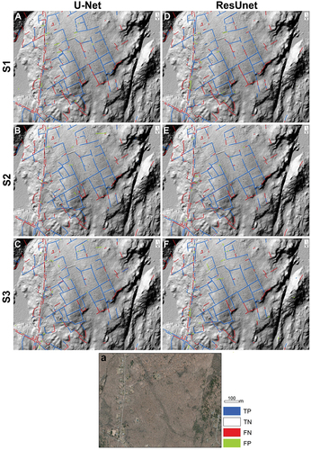
Figure 10. Examples of commission errors caused by morphological similarity on LiDAR hillshade surface. (A: example of wall-like features (a field edge with a pile of leaves) appearing on the hillshade map in the test site 1; B: U-Net S3 accuracy assessment result is overlayed on ; C: example of edge of trail in the test site 1; D: U-Net S3 accuracy assessment result is overlayed on ; E: example of road or curb edge in the test site 2; F: ResUnet S3 accuracy assessment result is overlayed on ). G: high-resolution orthophotography (CT ECO, 2019). Note that we used the best accuracy assessment result for each test site in this figure and background image is NW hillshade map. Note that TN symbol is transparent.
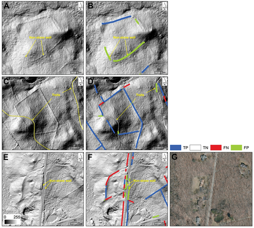
Figure 11. Example of omission error for S1 in test site 1 caused by alignment for direction of sunlight and stone walls. (A: stone walls in NW-SE direction are invisible in the NW hillshade map; B: stone walls in NW-SE direction are visible in the NE hillshade map; C: U-Net S1 accuracy assessment result is overlayed on ). Note that TN symbol is transparent.
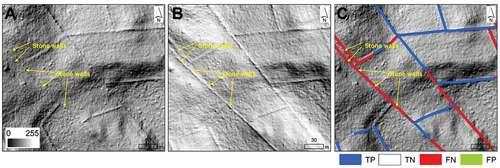
Figure 12. Example of omission error in test site 2 caused by darkness or brightness on the hillshade map. (A: stone walls disappear due to shade or low signal in NW hillshade map; B: stone walls appear unclear due to shade or low signal in NE hillshade map; C: ResUnet S3 accuracy assessment result is overlayed on ). Note that TN symbol is transparent.
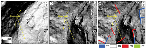
Figure 13. Example of poor-quality LiDAR hillshade image due to stone walls under canopy cover in Eastford town, CT. (A&D: NE hillshade map; B&E: U-Net S3 accuracy assessment result; C&F: photos taken from field work). Note that TN symbol is transparent.
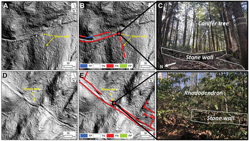
Figure 14. Stone wall mapping result in Cornwall town, CT (A: elevation map; B: 30m resolution land use/land cover map of 2015 (data source: (Center for Land Use Education & Research CT CLEAR. Citation2016)); C: Manually digitized SW result without post-processing (no PP); D: Manually digitized SW result after impervious cover post-processing (IC PP); E: Manually digitized SW result after impervious cover land cover post-processing (IC LC PP); F: U-Net S3 prediction result without post-processing (no PP); G: U-Net S3 prediction result after impervious cover post-processing (IC PP); H: U-Net S3 prediction result after impervious cover land cover post-processing (IC LC PP); I: ResUnet S3 prediction result without post-processing (no PP); J: ResUnet S3 prediction result after IC PP; K: ResUnet S3 prediction result after IC LC PP).
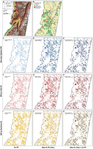
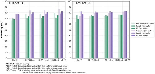
Figure 15. Accuracy assessment results of U-Net S3 and ResUnet S3 for town-level stone wall mapping.
Data availability statement
LiDAR data that used for this study are available upon request by contact with the corresponding author, or accessed through https://cteco.uconn.edu/data/download/flight2016/index.htm.