Thin cloud correction method for visible remote sensing images using a spectral transformation scheme

Figures & data

Figure 1. Correlation analysis among the visible bands of thin cloud image with different land covers: (a) observed thin cloud images, (b)–(d) band correlation analysis results of (a).

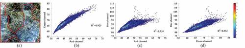
Figure 2. DCP maps estimated from the corresponding images $I_{\hspace{0.17em}}^{T_1}$and $I_{\hspace{0.17em}}^{T_2}$: (a)–(c) red (or red-like) bands of the original cloud-covered image and the two transformed images $I_{\hspace{0.17em}}^{T_1}$ and $I_{\hspace{0.17em}}^{T_2}$, (d)–(f) corresponding DCP maps estimated from the three images.

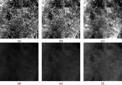
Figure 3. Procedure of the proposed scheme to estimate spatially varied atmospheric light: (a) patch division, (b) searching for dark object pixels in local patches, (c) estimated uneven atmospheric light.

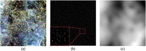
Figure 4. Comparison of the recovered results in the simulated experiment based on Landsat 8 OLI: (a) simulated cloud-covered image; (b)–(f) recovered results from HOT, HTM, TDCP, SpA-GAN, and the proposed method; (g) ground truth.

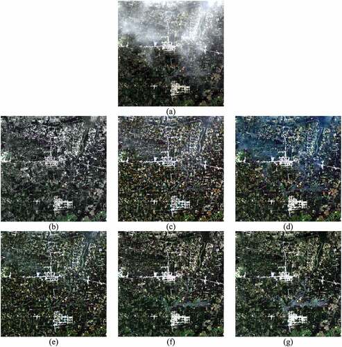
Table 1. Quantitative results of the four methods in the Landsat-based simulated data.

		HOT	HTM	TDCP	SpA-GAN	Proposed
Figure 4	R^2	0.6426	0.5583	0.8811	0.9421	0.9664
	RMSE	9.0707	11.9219	3.9321	2.2673	1.7380
	SA	3.2460	1.5115	1.5001	0.9916	0.7593

Figure 5. Comparison of the recovered results in the simulated experiment based on GaoFen-2: (a) simulated cloud-covered image; (b)–(f) recovered results from HOT, HTM, TDCP, SpA-GAN, and the proposed method; (g) ground truth.

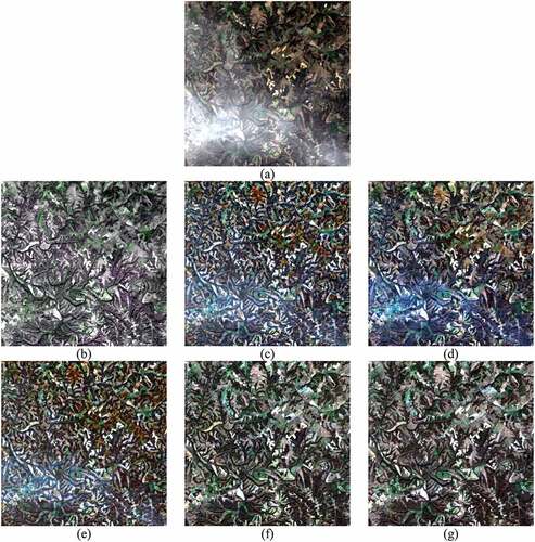
Table 2. Quantitative results of the four methods in the GaoFen-2-based simulated data.

		HOT	HTM	TDCP	SpA-GAN	Proposed
Figure 5	R^2	0.6411	0.6465	0.8360	0.8796	0.9791
	RMSE	10.6128	8.6219	3.3265	4.1671	0.9871
	SA	3.3608	1.3788	3.1053	2.4133	0.8870

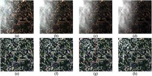
Figure 6. Comparison of recovered results in the first real data: (a) thin cloud image; (b)–(f) recovered results from HOT, HTM, TDCP, SpA-GAN, and the proposed method.

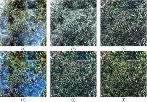
Figure 7. Transmission maps used in TDCP and the proposed method and their difference maps: (a) transmission map in TDCP, (b)–(d) transmission maps in the proposed method, (e)–(g) difference maps between (b)–(d) and (a).

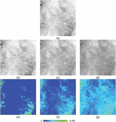
Figure 8. Comparison of recovered results in the second real data: (a) thin cloud image; (b)–(f) recovered results from HOT, HTM, TDCP, SpA-GAN, and the proposed method.

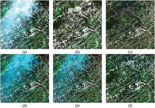
Figure 9. Comparison of recovered results in the fifth real data: (a) thin cloud image; (b)–(f) recovered results from HOT, HTM, TDCP, SpA-GAN, and the proposed method; (g) cloud-free image acquired temporally adjacent to (a).

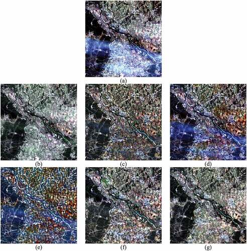
Table 3. Quantitative results of the four approaches in the fifth real data.

			RMSE	R^2	SA
Figure 9	HOT	Red	7.4211	0.6143	1.2143
		Green	8.9114	0.8162
		Blue	8.8453	0.7651
	HTM	Red	5.0133	0.7641	0.7622
		Green	5.5411	0.8321
		Blue	6.3654	0.8896
	TDCP	Red	4.5614	0.8825	0.8146
		Green	6.6631	0.8151
		Blue	7.1002	0.8162
		Red	4.9121	0.8246
	SpA-GAN	Green	6.1746	0.8119	0.8011
		Blue	6.2449	0.8473
	Proposed	Red	2.4711	0.8906	0.3912
		Green	2.1649	0.9147
		Blue	2.0189	0.9469

Figure 10. Comparison of recovered results in the sixth real data: (a) full-scene thin cloud-covered image, (b) recovered result from the proposed method.

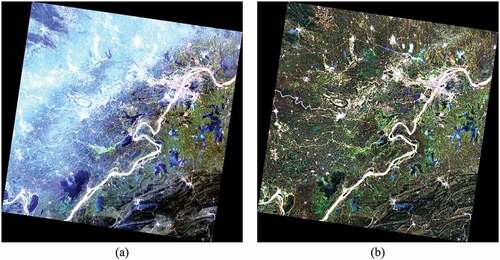
Figure 11. Real visible image captured by Landsat 8 OLI (path/row: 019/037) on May 12, 2022.

Figure 12. Four simulated thin cloud images with different cloud cover rates. The first row is the simulated thin cloud images, the second row is the ground truths of transmission maps, and the third row shows the corrected results using the proposed method.

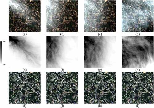
Figure 13. Four simulated thin cloud images with different cloud thicknesses. The first row is the simulated thin cloud images, and the second row shows the corrected results using the proposed method.

Data availability statement

Landsat 7 ETM+ and Landsat 8 OLI images are available from USGS (https://earthexplorer.usgs.gov/). GaoFen-2 images are available and can be accessed from http://www.cresda.com/CN/.