The essence of acquisition time of airborne hyperspectral and on-ground reference data for classification of highly invasive annual vine Echinocystis lobata (Michx.) Torr. & A. Gray

Figures & data

Figure 1. Development phases of Echinocystis lobata in A) spring (May), B) summer (July), and C) autumn (September).

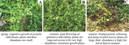
Figure 2. Location of the study area and distribution of the reference polygons (based on the Digital Terrain Model), highlighting planned flight paths in the study area (based on the RGB orthophoto map).

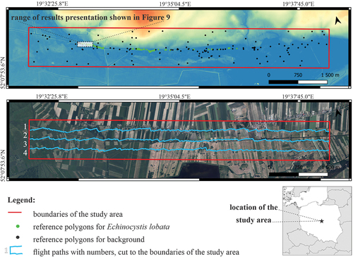
Figure 3. Diagram showing the process of preparing hyperspectral data from three single flights (spring, summer, autumn) to multitemporal data fusion.

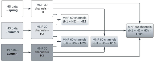
Figure 4. Examples of changing the location of reference polygons in subsequent measurement campaigns (A – spring, B – summer, C – autumn), in relation to the direction of plants’ shoots growth.

Figure 5. A flowchart of the classification process.

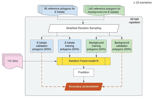
Figure 6. Mean spectral signatures of Echinocystis lobata and 8 background subclasses (abbrv.: ech_lob - Echinocystis lobata; cal_sep - Calystegia sepium; cir_arv - Cirsium arvense; hum_lup - Humulus lupulus; phr_aus - Phragmites australis; urt_dio - Urtica dioica) from hyperspectral images and reference polygons from: (A) spring; (B) summer, and (C) autumn campaigns. Wavelength ranges where the reflectance coefficient differed significantly for Echinocystis lobata against the remaining subclasses (except Calystegia sepium, Humulus lupulus) are shown in grey (Kruskal-Wallis test: n.S., α = 0.05).

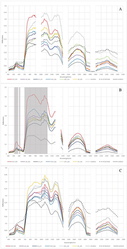
Figure 7. Mean spectral signatures of Echinocystis lobata in spring (A), summer (B), and autumn (C) campaigns from hyperspectral images using reference polygons. Wavelength ranges where the reflectance coefficient differed significantly for spring, summer and autumn are shown in grey (Kruskal-Wallis test: n.S. α = 0.05).

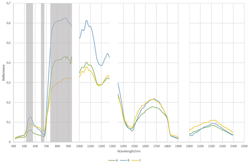
Figure 8. The comparison of scenarios R1H1, R2H2 and R3H3 according to F1 values for Echinocystis lobata for a given scenario. Boxplots were created from fifty Random Forest classifications for each scenario. Line – indicates the average value; box – represents the first and the third quartile; plot – the highest and the lowest values in each scenario. Abbreviations: on-ground data collection in: R1 (spring), R2 (summer), R3 (autumn). Airborne hyperspectral data acquisition: H1 (spring), H2 (summer), H3 (autumn). ANOVA was used to test the significance of the difference between the scenarios. Based on the post-hoc Tukey’s tests, scenarios between which there is no difference were marked with the same letter.

Figure 9. Echinocystis lobata classification results in three scenarios: spring (R1H1), summer (R2H2), and autumn (R3H3). The localisation of this area is marked in Figure 2.

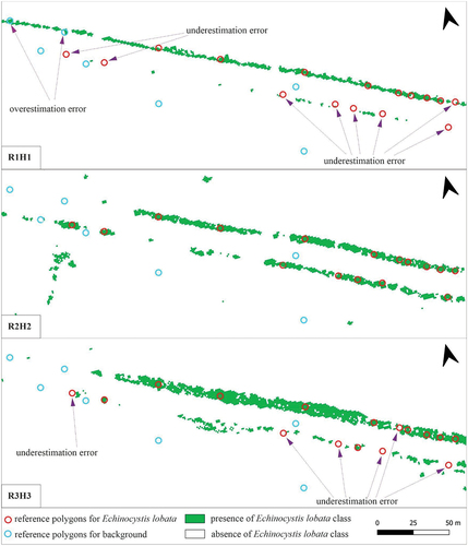
Table 1. The comparison of average accuracy obtained from classification for three scenarios: R1H1, R2H2, and R3H3, according to values: OA – overall accuracy, F1 for Echinocystis lobata and F1 for background class. Abbreviations: on-ground data collection in: R1 (spring), R2 (summer), R3 (autumn). Airborne hyperspectral data acquisition: H1 (spring), H2 (summer), H3 (autumn).

Scenario	Class	OA - mean ± SD	F1 - mean ± SD
R1H1	E. lobata	0.93 ± 0.01	0.64 ± 0.04
	Background		0.96 ± 0.01
R2H2	E. lobata	0.97 ± 0.01	0.87 ± 0.04
	Background		0.99 ± 0.01
R3H3	E. lobata	0.95 ± 0.01	0.75 ± 0.05
	Background		0.98 ± 0.01

Figure 10. The comparison of scenarios R1H1 with R2H1 and R3H1; R2H2 with R1H2 and R3H2; and R3H3 with R1H3 and R2H3 according to F1 values for Echinocystis lobata for a given scenario. Boxplot was created from fifty Random Forest classifications. Line – indicates the average value; box – represents the first and the third quartile; plot – the highest and the lowest values in each scenario. Abbreviations: on-ground data collection in: R1 (spring), R2 (summer), R3 (autumn). Airborne hyperspectral data acquisition: H1 (spring), H2 (summer), H3 (autumn). ANOVA was used to test the significance of the difference between the scenarios. Based on the post-hoc Tukey’s tests, scenarios between which there is no difference were marked with the same letter.

Table 2. The comparison of scenarios R1H1 with R2H1 and R3H1; R2H2 with R1H2 and R3H2; and R3H3 with R1H3 and R2H3 according to values: OA – overall accuracy, F1 for Echinocystis lobata and F1 for background class. Abbreviations: on-ground data collection in: R1 (spring), R2 (summer), R3 (autumn). Airborne hyperspectral data acquisition: H1 (spring), H2 (summer), H3 (autumn).

Accuracy measures	Reference scenario		The differences between reference scenarios
			R2H1	R3H1
OA	R1H1	0.93 ± 0.01	−0.01	−0.02
F1 - E. lobata		0.64 ± 0.04	−0.04	−0.08
F1 - Background		0.96 ± 0.01	−0.01	−0.01
			R1H2	R3H2
OA	R2H2	0.97 ± 0.01	−0.04	−0.04
F1 - E. lobata		0.87 ± 0.04	−0.07	−0.05
F1 - Background		0.99 ± 0.01	−0.01	−0.01
			R1H3	R2H3
OA	R3H3	0.95 ± 0.01	−0.02	−0.02
F1 - E. lobata		0.75 ± 0.05	−0.02	+0.01
F1 - Background		0.98 ± 0.01	−0.01	−0.01

Figure 11. The comparison of scenarios R1H1 with R1H12, R1H13 and R1H123; R2H2 with R2H12, R2H23 and R2H123; and R3H3 with R3H13, R3H23 and R3H123 according to F1 values for Echinocystis lobata for a given scenario. Boxplot was created from fifty Random Forest classifications. Line – indicates the average value; box – represents the first and the third quartile; plot – the highest and the lowest values in each scenario. Abbreviations: on-ground data collection in: R1 (spring), R2 (summer), R3 (autumn). Airborne hyperspectral data acquisition: H1 (spring), H2 (summer), H3 (autumn). ANOVA was used to test the significance of the difference between the scenarios. Based on the post-hoc Tukey’s tests, scenarios between which there is no difference were marked with the same letter.

Table 3. The comparison of scenarios R1H1 with R1H12, R1H13, and R1H123; R2H2 with R2H12, R2H23, and R2H123; and R3H3 with R3H13, R3H23, and R3H123 according to values: OA – overall accuracy, F1 for Echinocystis lobata and F1 for background class. Abbreviations: on-ground data collection in: R1 (spring), R2 (summer), R3 (autumn). Airborne hyperspectral data acquisition: H1 (spring), H2 (summer), H3 (autumn).

Accuracy measures	Reference scenario		The differences between reference scenarios
			R1H12	R1H13	R1H123
OA	R1H1	0.93 ± 0.01	+0.04	+0.03	+0.04
F1 - E. lobata		0.64 ± 0.04	+0.20	+0.13	+0.22
F1 - Background		0.96 ± 0.01	+0.02	+0.01	+0.03
			R2H12	R2H23	R2H123
OA	R2H2	0.97 ± 0.01	+0.01	−0.01	+0.01
F1 - E. lobata		0.87 ± 0.04	+0.01	+0.03	+0.04
F1 - Background		0.99 ± 0.01	0.00	0.00	0.00
			R3H13	R3H23	R3H123
OA	R3H3	0.95 ± 0.01	+0.01	+0.02	+0.02
F1 - E. lobata		0.75 ± 0.05	+0.03	+0.12	+0.11
F1 - Background		0.98 ± 0.01	0.00	+0.01	0.00

Data availability statement

The hyperspectral data used in the study were acquired as part of the HabitARS project and can be made available upon request by Consortium Leader MGGP Aero. The polygons used in the training and validation of the models are available here: https://data.mendeley.com/datasets/kx47c9r5tt.