
Figures & data
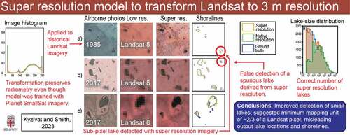
Figure 1. Study regions are derived from available HR vector lake maps created for the NASA Arctic-Boreal Vulnerability Experiment (ABoVE) (Kyzivat et al. Citation2018, Citation2019; in red); and a historical study of permafrost lake change (Walter Anthony et al. Citation2021, in blue).
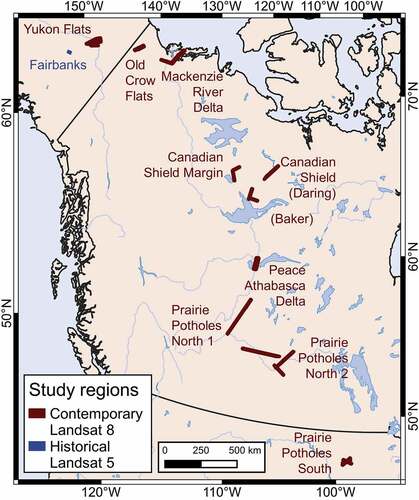
Figure 2. Sensitivity test for standard deviation of Gaussian smoothing kernel used for image reconstruction varying from 2 pixels (a) to 1,000 pixels (g). Seamlines are visible near the image center-left and and/or center-bottom for all standard deviation values except 10 and 100, so an intermediate value of 30 was chosen. Center coordinates are 52.6563° N, 107.08323° W. Panel (d) illustrates of the weights of a single kernel, and (h) illustrates the superposition of multiple kernels, used to normalize the resulting image. Panels (d) and (h) are 480 pixels square and are schematics not associated with a particular geographic location.
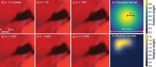
Figure 3. Flow chart of image processing, super resolution transformation, classification and overlap analysis. Inputs are in teal parallelograms, analyses are in green diamonds, and models are in red circles. HR refers to high resolution, LR to low resolution, and GT to ground truth.
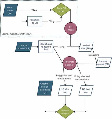
Figure 4. Example pixel frequencies for Yukon Flats, Alaska (a-c), Canadian Shield near Baker Creek (d-f), and Fairbanks, AK 1985 (g-i). Bin counts are normalized to facilitate comparison between data sets of different sizes. Jagged Landsat 5 histograms are a result of the 1–95% image stretch applied to native 8-bit radiometric resolution. In contrast, the SR transformation produces smooth histograms that make use of the total dynamic range.
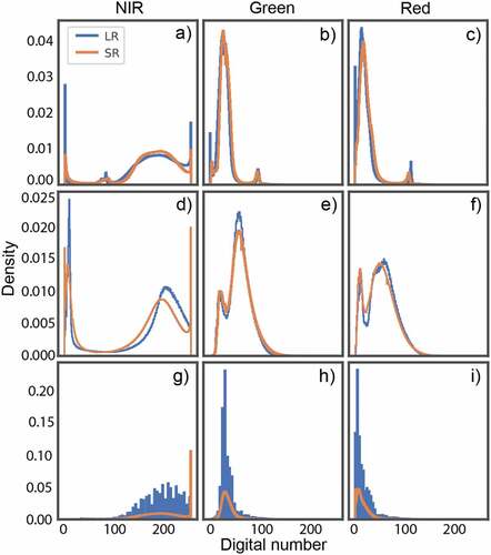
Figure 5. Airborne camera GT and Landsat LR and SR examples demonstrate the advantages and limitations of SR in Fairbanks, Alaska, 1985 (a); Prairie Potholes South, North Dakota (b); Canadian Shield Margin, Northwest Territories (c); Mackenzie River Delta, Northwest Territories (d); and Old Crow Flats, Yukon territories (e). In row (a), an additional lake is detected in SR compared to LR for Landsat 5 data from 1985. In (b), the lake in the northeast corner has an SR lake detection within thirty meters of GT, showing how use of an adjacency buffer better evaluates results. Several lakes fragmented into two in the SR classification, altering the abundance but not total area of lakes. In row (c), SR classification detects one lake missed in LR, but both classifiers miss three lakes sized near the native GT MMU. In row (d), several small GT lakes are not detected in either Landsat resolution. A river in the top of the image is successfully masked out and therefore does not contribute to summary metrics. In row (e), all lakes detected in SR are also detected in LR, and there are two false positive SR lakes generated near the image center. Center coordinates: 64.8775, −147.7242 (a); 47.1432, −99.2494 (b); 63.7498, −117.6939 (c); 68.2699, −134.4791 (d); 67.8731, −139.9617 (e).
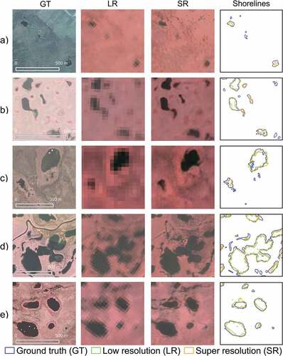
Figure 6. Accuracy metrics for different minimum lake sizes indicate that recall and F-1 scores are greater for Landsat SR than LR for all lake sizes (e, f), while precision varies and is less for SR than LR for small lakes until a transition at 1,000 m2 (d). An effective MMU of 500 m2 (2/3 of a Landsat pixel) is determined based on the global maximum of F-1 score in (c). Metrics are calculated against all GT lakes (a-c), and for GT lakes only above the corresponding lake size threshold (d-f), with the latter curves being noisier due to the sample size decreasing with size threshold. The precision-recall curve (g) is plotted using data in (d-f), and the SR classification has a greater area under the curve (0.57) than that of LR (0.48).
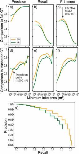
Table 1. SR lake detections have better skill than LR for lakes larger than 500 m2, as measured by Average Recall (AR) and F-1 score (AF1), but not by Average Precision (AP), when compared against GT.
Figure 7. Lake-size distribution histograms based on all detected lakes (a, c) show good agreement between the size frequencies of SR and GT lakes for contemporary Landsat 8 scenes (a, b) and historical Landsat 5 scenes (c, d). When only plotting true positive lakes (b, d), this agreement is diminished, although SR still detects more lakes than LR in nearly all size bins up to 10,000 m2 for both recent (b) and 1985 (d) Landsat imagery. Removing rivers occasionally led to LR lakes counterintuitively smaller than one 900 m2 Landsat pixel (a, b). These lakes were nevertheless retained to follow consistent geoprocessing steps for all datasets.
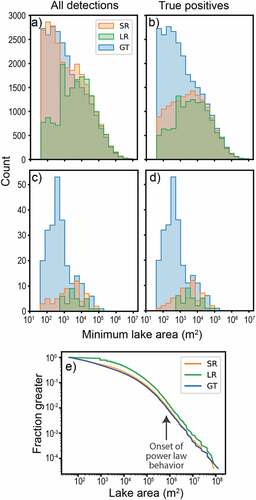
Figure 8. Accuracy metrics for different tolerance distances to 90 m based on the MMU of 500 m2. reports mean statistics using tolerances ≤ 30m.
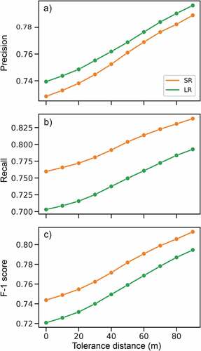
Table 2. Scale-independent lake detection metrics of count (N), true positives, lake area, and power law parameters A0 (optimal onset of power law behavior) and α (fitted power law slope).