
Figures & data
Figure 1. Schematic diagram of BWS-DIE algorithm.
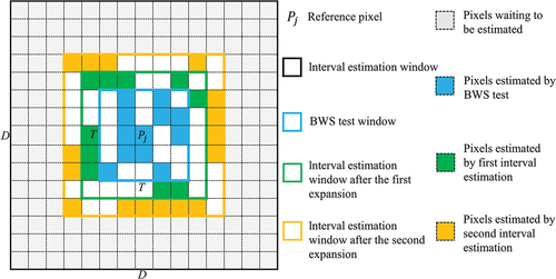
Figure 2. Flow chart of BWS-DIE algorithm.
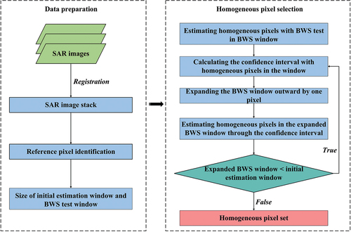
Figure 3. BWS-DIE MT InSAR processing flow.
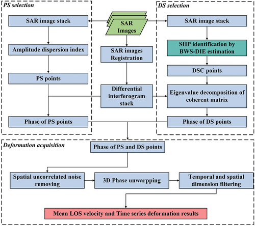
Figure 4. Also show that, when the sample numbers differ, 4(a-f) as the contrast of K1/K2 increases, and when the difference between homogeneous pixels and heterogeneous pixels becomes increasingly obvious, the rejection means for all of the algorithms can converge to the vicinity of the real power. However, when the sample numbers differ, each algorithm performs differently. In (), when the contrast of K1/K2 is 1–1.4 (the power value does not reach the convergence state), the rejection mean of the KS algorithm is lower than the rejection means of the BWS, FaSHPS and BWS-DIE algorithms. This finding indicates that, when the difference between homogeneous pixels and heterogeneous pixels is not significant, the KS algorithm is at its lowest performance level. The BWS algorithm slightly outperforms the KS algorithm, but () clearly indicates that its performance is relatively poor for small samples and that it is close to the real power value until the contrast of K1/K2 exceeds 2.2. This finding indicates that the BWS algorithm increases the type II error for small samples and is prone to contain a greater number of heterogeneous samples.
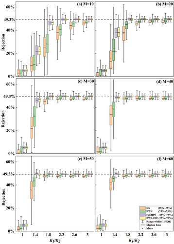
Table 1. Comparison of performance results for different homogeneous pixel algorithms. Note that all data were collected in the convergence state of power value (i.e. the contrast of K1/K2 is 3).
Figure 5. Location and mine distribution in research area, as modified from Chen et al. (Citation2022) [remote sensing]. (a) Location map of research area. (b) Mine boundaries and distributions of some working panels. Red triangle represents Xuzhou – the research area. Red dots represent fourth-class leveling monitoring points for a total of ten points. Note that leveling data were collected using an OPTONS3 electronic level with accuracy of ±3 mm per kilometer round trip. (c), (d) and (e) are enlarged drawings of working panels of Zhangxiaolou, Jiahe and Pangzhuang mines, respectively..
![Figure 5. Location and mine distribution in research area, as modified from Chen et al. (Citation2022) [remote sensing]. (a) Location map of research area. (b) Mine boundaries and distributions of some working panels. Red triangle represents Xuzhou – the research area. Red dots represent fourth-class leveling monitoring points for a total of ten points. Note that leveling data were collected using an OPTONS3 electronic level with accuracy of ±3 mm per kilometer round trip. (c), (d) and (e) are enlarged drawings of working panels of Zhangxiaolou, Jiahe and Pangzhuang mines, respectively..](/cms/asset/af29686a-1333-4b38-8e9e-39019bd01c86/tgrs_a_2218261_f0005_oc.jpg)
Table 2. Working panel information.
Table 3. SAR image parameters. The perpendicular and temporal baselines are calculated based on the reference image.
Figure 6. Spatial-temporal baseline distributions of interferometric pairs. The red dot represents the acquisition data of reference image.
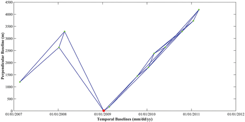
Figure 7. Average annual subsidence velocity in line-of-sight (LOS) direction in research area. (a) Average annual subsidence velocity obtained using BWS-DIE MT InSAR method. (b) Average annual subsidence velocity obtained using StaMPS method. Note that in (a) and (b), white circles A, B, C, D, E, F, G and H indicate areas with drastic deformation; significant differences in results were obtained using both methods.
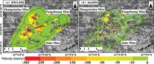
Figure 8. Time series cumulative subsidence obtained by BWS-DIE algorithm for research area in LOS direction. A, B and C indicate areas with significant subsidence.
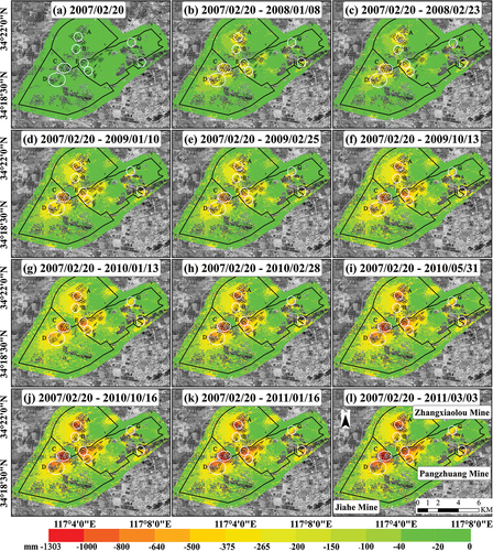
Figure 9. Time series cumulative subsidence obtained by StaMPS method for research area in LOS direction. A, B and C indicate areas with significant subsidence.
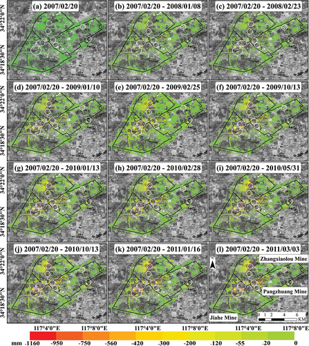
Figure 10. Comparisons of different monitoring results. (a) Comparison of subsidence values obtained using BWS-DIE MT InSAR and StaMPS algorithms with fourth-order leveling results. (b) RMSE and correlation coefficients calculated from subsidence results and leveling data obtained using BWS-DIE MT InSAR algorithm. (c) RMSE and correlation coefficients calculated from subsidence results and leveling data obtained using StaMPS algorithm.
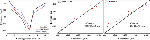
Figure 11. SAR intensity image of research area. Yellow circle K indicates typical area covered by bare land, farmland and sparse vegetation, and yellow circle I indicates area where dense buildings are located. J, L and M are feature points of buildings, roads and vegetation, respectively.
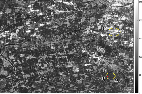
Figure 12. Comparison of results of selection numbers obtained using different homogeneous pixel algorithms. (a-d) are homogeneous pixel selection results obtained using BWS-DIE, KS, BWS and FaSHPS algorithms, respectively. Areas covered by white circles I and K are buildings and vegetation coverage areas, respectively. Color scale means number of homogeneous pixels for each pixel.
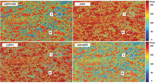
Figure 13. Results comparing the number of homogeneous pixels according to different homogeneous pixel selection methods and different reference pixels. (a-d) show number of homogeneous pixels obtained using BWS-DIS, KS, BWS and FaSHPS algorithms, respectively, when reference pixel is J. Red dots indicate reference pixels, and the pixel is located in building area. Yellow dots indicate the results of selecting homogeneous pixels. (e-h) are number of homogeneous pixel samples obtained using BWS-DIS, KS, BWS and FaSHPS algorithms when reference pixel is L. Red dots indicate reference pixels and the pixel being located on a road; yellow dots indicate results of homogeneous pixel selection. (i-l) show number of homogeneous pixel samples obtained using BWS-DIS, KS, BWS and FaSHPS algorithms, respectively, when reference pixel is M. Red dots indicate reference pixels, and pixel is located in vegetation area. Yellow dots indicate results from homogeneous pixel selection.
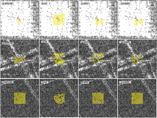
Figure 14. Annual average subsidence velocities obtained by different homogeneous pixel algorithms for research area along LOS direction. (a-d) show annual average subsidence velocities obtained by BWS-DIE, KS, BWS and FaSHPS algorithms for research area, respectively. White circle N indicates area with largest annual average velocity obtained by different homogeneous pixel algorithms.
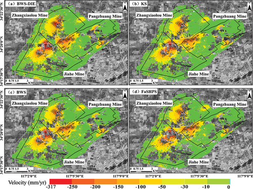
Figure 15. Average annual subsidence velocities and densities of common points of results of different algorithms. (a) LOS displacement velocity derived using KS algorithm versus BWS-DIE algorithm. (b) LOS displacement velocity derived using BWS algorithm versus BWS-DIE algorithm. (c) LOS displacement velocity derived using FaSHPS algorithm versus BWS-DIE algorithm. Results are colour-coded according to pixels’ smoothed density (Eilers and Goeman Citation2004), in which red represents the greatest dot density and blue represents the least dot density.
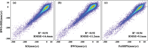
Figure 16. Histogram of deformation velocities derived by different methods. (a) BWSDIE algorithm versus KS algorithm. (b) BWS-DIE algorithm versus BWS algorithm. (c) BWS-DIE algorithm versus FaSHPS algorithm.
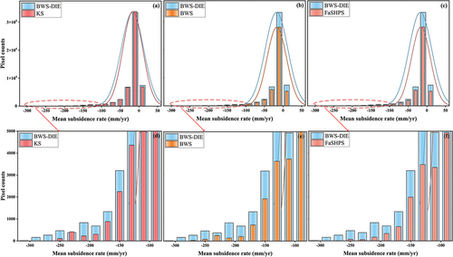
Figure 17. Cumulative subsidence of research area for period February 20, 2007 to March 3, 2011, when different homogeneous pixel algorithms were employed. (a-c) show cumulative subsidence obtained by BWS-DIE algorithm; (d-f) show cumulative subsidence obtained by KS algorithm; (g-i) show cumulative subsidence obtained by BWS algorithm; and (j-l) show cumulative subsidence obtained by FaSHPS algorithm. Red circles O and P indicate areas with different local surface deformation characteristics obtained by algorithms from February 20, 2007 to January 10, 2009, and red circle N indicates area with largest surface subsidence value.
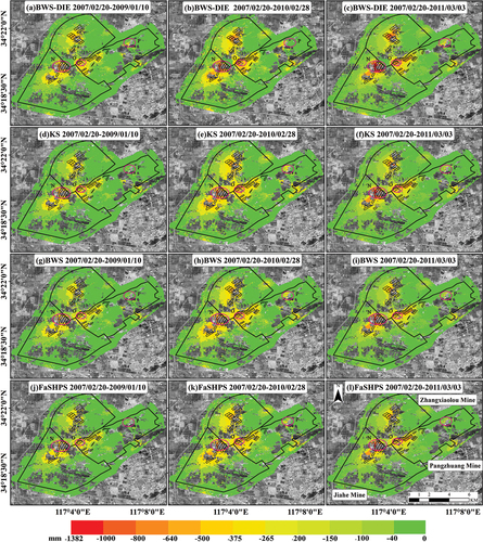
Figure 18. Time series cumulative subsidence results of areas covered by red dotted circle O from February 20, 2007 to January 10, 2009, when different algorithms were employed. Black polygon represents working panel No. 15..
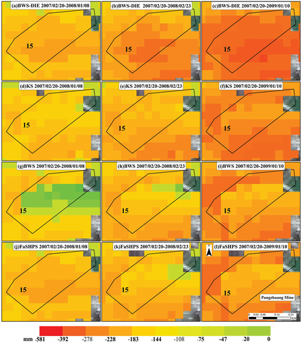
Figure 19. Cumulative subsidence results of areas covered by red dotted circle P from February 20, 2007 to January 10, 2009, when different algorithms were employed.
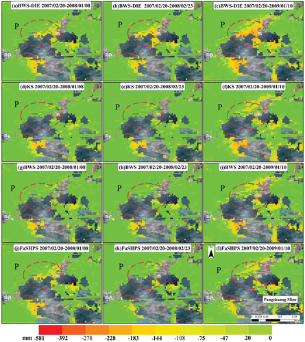
Figure 20. The Google images between March 2017 and October 2012. The irregular polygon formed by the blue curved line represents the area of the lake.
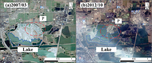
Figure 21. (a-h) is deformation time series comparison results; (i-l) is statistical comparison results between the different algorithms.
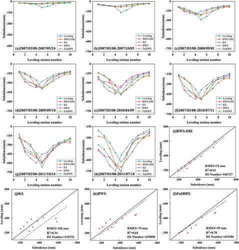
Table 4. Runtime of different algorithms.
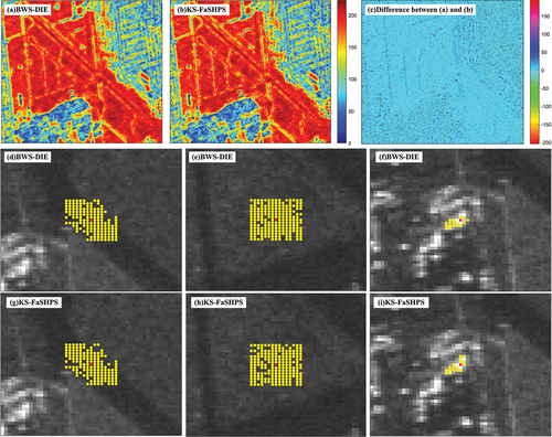
Figure 22. Comparison of homogeneous pixel selection results between BWS-DIE and KS- FaSHPS. It is noticed that red dots indicate reference pixels and yellow dots indicate results of homogeneous pixel selection; the reference pixels are located in road, bare land and building areas in Figures 22(d-g), (e-h) and (f-i), respectively.
Data availability statement
The MATLAB codes for Monte Carlo simulation experiment, Phase optimization and BWS-DIE algorithm are available at https://github.com/Ming-subsidence/time-series-deformation.