Local-aware coupled network for hyperspectral image super-resolution

Figures & data

Figure 1. Overview of the proposed local-aware coupling network (LCNet). The proposed framework includes a simulated data generation module for input data and SRF calculation, an LR HSI reconstruction network designed for learning spectral feature recovery, and an HR MSI reconstruction network with spatial local-aware block for capturing key region features. The output target image is generated by the HR MSI reconstruction network.

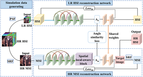
Figure 2. The spatial feature loss challenge of fusion-based HSI SR. The number of bands L in HSI is much larger than the number of basis vectors p, as well as the number of bands l in MSI. When mapping spatial features to more bands during image fusion, it is easy to cause loss of information.

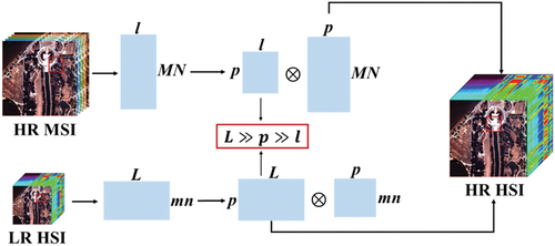
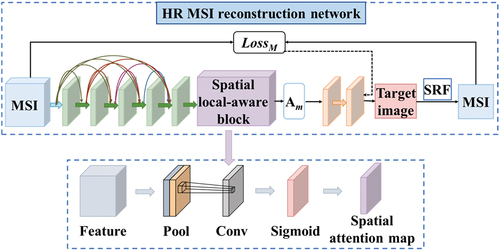
Figure 3. Spatial local-aware block. After feature extraction through a densely connected structure, the MSI is fed into the module. After pooling, convolution, and activation, a spatial attention map is obtained, which aims to focus on the texture structures of key regions.

Table

Algorithm 1: LCNet Algorithm

Input: HR MSI $\mathbf{Y}$ LR HSI $\mathbf{Z}$ Output: Reconstructed HR HSI $\widehat{X}$ 1: Input $\mathbf{Z}$ to train the LR HSI reconstruction network to obtain the decoder weights ${\theta }_{hd}$. 2: Calculate $L({\theta }_{he},{\theta }_{hd})=\frac{1}{2}{\Vert Z({\theta }_{he},{\theta }_{hd})-\widehat{Z}({\theta }_{he},{\theta }_{hd})\Vert }_F^2+\lambda H(A_h({\theta }_{he}))+\mu {\Vert {\theta }_{hd}\Vert }_F^2$ 3: Repeat and obtain the decoder weights ${\theta }_{hd}$ 4: Input $\mathbf{Y}$ and use the shared decoder weight ${\theta }_{hd}$ to update the encoder weights ${\theta }_{md}$ of the LR HSI reconstruction network. 5: Calculate $L({\theta }_{me})=\frac{1}{2}{\Vert Y({\theta }_{me},{\theta }_{hd})-\widehat{Y}({\theta }_{me},{\theta }_{hd})\Vert }_F^2+\lambda H(A_h({\theta }_{me}))$ 6: Calculate the following formula every 10 iterations. $\mathcal{A}\left({\tilde{\mathbf{A}}}_h,{\mathbf{A}}_m\right)=\frac{1}{MN}(\sum _{i=1}^{MN}arccos(\frac{{{\tilde{\mathbf{A}}}^i}_h\cdot {\mathbf{A}}_m^i}{{∥{{\tilde{\mathbf{A}}}^i}_h∥}_2{∥{\mathbf{A}}_m^i∥}_2}))$ 7: repeat 8: until Convergence 9: return Target HR HSI $\widehat{X}$

Figure 4. The color-composite of three public hyperspectral datasets. (a) Indian Pines, (b) Pavia University and (c) Washington DC.

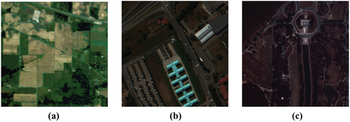
Table 1. The ability of each method to learn unknown SRF and PSF.

	SFIM	GLPHS	GSA	CNMF	FUSE	HySure	CSTF	uSDN	LCNet
SRF	×	×	×	×	×	√	×	×	√
PSF	×	×	×	×	×	√	×	̶	√

Figure 5. Grayscale display comparison of the 5th band of the reconstruction results on the Indian Pines data. Methods: (a) SFIM, (b) GLPHS, (c) GSA, (d) CNMF, (e) FUSE, (f) HySure, (g) CSTF, (h) uSDN, (i) LCNet, (j) Reference image.

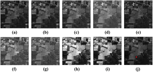
Figure 6. Comparison of the error maps of the 5th band of the reconstruction results on the Indian Pines data. Methods: (a) SFIM, (b) GLPHS, (c) GSA, (d) CNMF, (e) FUSE, (f) HySure, (g) CSTF, (h) uSDN, (i) LCNet.

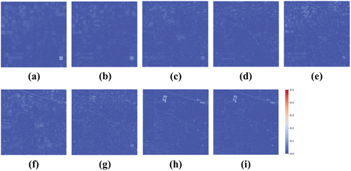
Figure 7. Spectral curves of each method at the red mark of Indian Pines data.

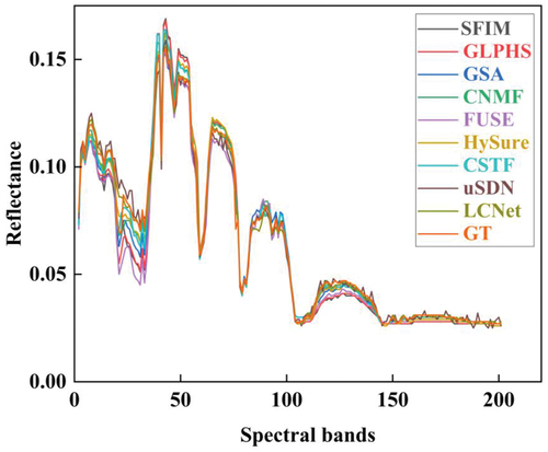
Table 2. Quantitative performance comparison of each method on the Indian Pines dataset. The best results are highlighted in bold.

	SFIM	GLPHS	GSA	CNMF	FUSE	HySure	CSTF	uSDN	LCNet
PSNR	30.252	31.931	32.715	32.760	30.226	34.180	35.210	35.668	37.544
SAM	3.042	2.699	2.748	2.487	3.221	2.889	2.778	2.388	1.700

Figure 8. Grayscale display comparison of the 30th band of the reconstruction results on the Pavia University data. Methods: (a) SFIM, (b) GLPHS, (c) GSA, (d) CNMF, (e) FUSE, (f) HySure, (g) CSTF, (h) uSDN, (i) LCNet, (j) Reference image.

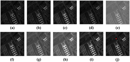
Figure 9. Comparison of the error maps of the 30th band of the reconstruction results on the Pavia University data. Methods: (a) SFIM, (b) GLPHS, (c) GSA, (d) CNMF, (e) FUSE, (f) HySure, (g) CSTF, (h) uSDN, (i) LCNet.

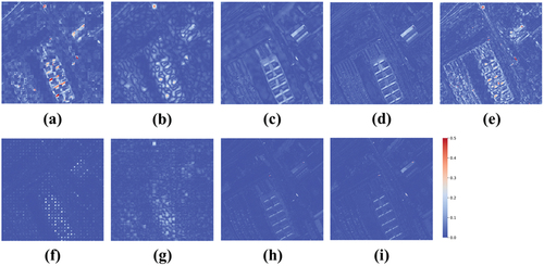
Figure 10. Spectral curves of each method at the red mark of Pavia University data.

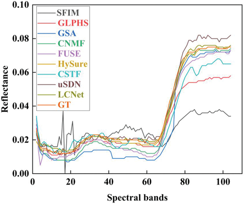
Table 3. Quantitative performance comparison of each method on the Pavia University data. The best results are highlighted in bold.

	SFIM	GLPHS	GSA	CNMF	FUSE	HySure	CSTF	uSDN	LCNet
PSNR	23.714	27.849	28.091	29.112	24.541	33.278	30.246	33.347	35.778
SAM	8.759	7.011	10.178	6.333	12.941	4.189	7.408	6.342	4.381

Figure 11. Grayscale display comparison of the 40th band of the reconstruction results on the Washington DC data. Methods: (a) SFIM, (b) GLPHS, (c) GSA, (d) CNMF, (e) FUSE, (f) HySure, (g) CSTF, (h) uSDN, (i) LCNet, (j) Reference image.

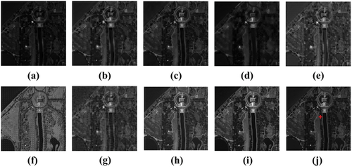
Figure 12. Comparison of the error maps of the 40th band of the reconstruction results on the Washington DC data. Methods: (a) SFIM, (b) GLPHS, (c) GSA, (d) CNMF, (e) FUSE, (f) HySure, (g) CSTF, (h) uSDN, (i) LCNet.

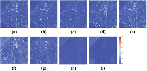
Figure 13. Spectral curves of each method at the red mark of Washington DC data.

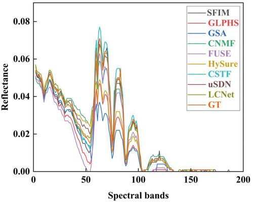
Table 4. Quantitative performance comparison of each method on the Washington DC data. The best results are highlighted in bold.

	SFIM	GLPHS	GSA	CNMF	FUSE	HySure	CSTF	uSDN	LCNet
PSNR	21.106	25.444	26.097	25.600	22.244	25.731	32.131	38.260	39.977
SAM	8.376	5.589	6.376	4.969	8.150	14.329	6.740	6.286	4.264

Figure 14. Grayscale display comparison of the 14th band of the reconstruction results on the real dataset. Methods: (a) LR HSI, (b) HR MSI (bands 3, 2, 1), (c) SFIM, (d) GLPHS, (e) GSA, (f) CNMF, (g) FUSE, (h) HySure, (i) uSDN, (j) LCNet.

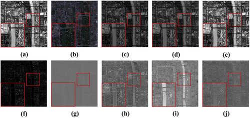
Table 5. Ablation and substitution experiment results on the Washington DC dataset. The best results are highlighted in bold.

Method	PSNR	SAM
LCNet-slb	36.811	6.086
LCNet-slb+CBAM	31.969	9.366
LCNet-slb+SE	38.047	5.059
LCNet	39.977	4.264

Table 6. Parameters and FLOPs of LCNet and uSDN on the Washington DC dataset.

Method	Params	FLOPs
uSDN	0.012M	16.717G
LCNet-slb	0.043M	20.774G
LCNet	0.048M	24.661G

Data availability statement

The Indian Pines, Pavia University, and Washington DC datasets are publicly available hyperspectral image datasets. The datasets can be downloaded from the following link: https://rslab.ut.ac.ir/data. The OHS-1 hyperspectral data can be obtained from the following link can be downloaded from the following link: https://www.orbitalinsight.com/data/. The GF-2 multispectral data can be downloaded from the following link: https://data.cresda.cn/.