
Figures & data
Figure 1. Overall structure of the proposed WISTE method. The encoder part is shown in the blue box, and the decoder part is shown in the green box. The Swin Transformer block structure is shown in the lower-right part. The abbreviations MLP, LN, W-MSA, and SW-MSA denote a multilayer perceptron, layer normalization, window-based multihead self-attention, and shifted window-based multihead self-attention, respectively.
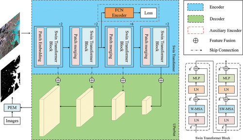
Figure 2. Main computation process of the Swin Transformer. (a) Patch merging to reduce the dimensionality of the feature map. The H, W, and C values of a patch denote the height, width, and number of channels of the corresponding feature map, respectively. (b) Hierarchical layer with different window sizes, with sampling levels of 4×, 8×, and 16×. (c) Window partitioning strategy in the Swin Transformer, where the semantic information between neighbouring patches is considered. (d) Shifted-window self-attention computation. The patches in dashed red boxes are masked, and self-attention is computed within the solid red boxes.
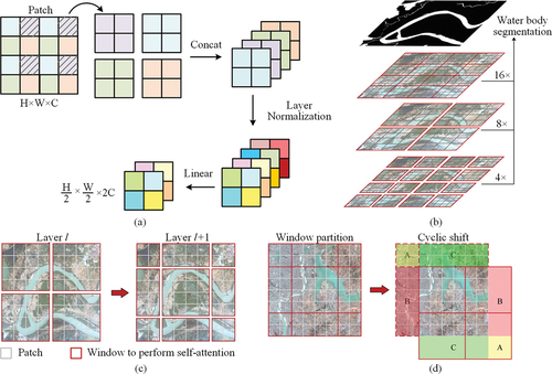
Figure 3. Illustration of the dual-encoder architecture of the WISTE. The auxiliary encoder branch is indicated by a dashed red box. ST denotes the Swin Transformer; Wi represents the matrices for each computational block; xi denotes the intermediate layer outputs; and Li signifies the loss function of the corresponding branch.
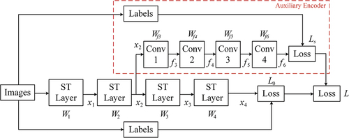
Figure 4. Images land cover labels and corresponding water body extraction labels of two public datasets, i.e. (a) The GID and (b) DeepGlobe dataset.
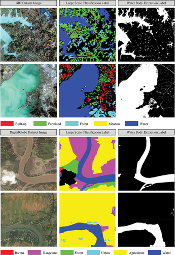
Figure 5. Images and labels of different water types contained in the GID dataset. From top to bottom, the rows present lakes, rivers, canals, and ponds.
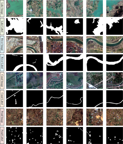
Figure 6. One Sentinel-2 image used for ablation experiments. (a) Sentinel-2 image obtained after band fusion (B2, B3, B4 and B8 for the B, G, R, and NIR bands, respectively). (b) Ground truth of the water body, with water in white and the background in black.
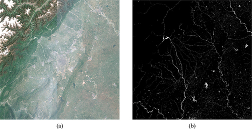
Table 1. Ablation experiment results obtained by the proposed WISTE on the GID and Sentinel-2 images (the best values are in bold).
Figure 7. Comparison among the prediction results produced by different methods on the DeepGlobe dataset. The water areas are in white, while the background is in black. The red boxes highlight areas with weak spatial information.
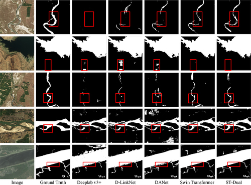
Table 2. Comparison among the different methods on the DeepGlobe dataset (the best values are in bold).
Figure 8. Comparison among the prediction results produced by different methods using the GID. The water areas are drawn in white. The areas where the WISTE demonstrates greater advantages are highlighted in red boxes.
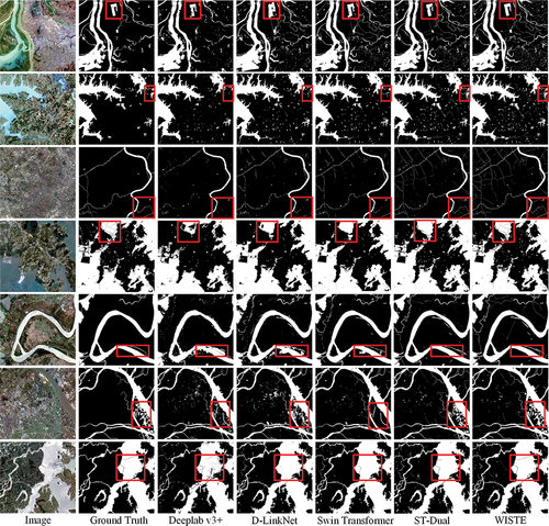
Table 3. Comparison among the different methods on the GID dataset (the best values are in bold).
Figure 9. In-detail comparison among the prediction results produced by different methods on the GID dataset.
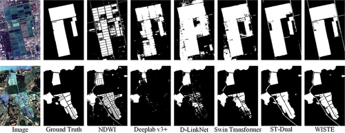
Table 4. Different band arrangements of the training samples in the GID dataset (the best values are in bold).
Table 5. Relationships between different FCN positions and the accuracy of ST-Dual (the best values are in bold).
Supplemental Material
Download MS Word (15.6 MB)Data availability statement
The datasets used in this study are publicly available. The Gaofen Image Dataset (GID) is available at https://x-ytong.github.io/project/GID.html, and the DeepGlobe dataset is downloadable at https://competitions.codalab.org/competitions/18468