
Figures & data
Figure 1. An example of an unidentified sub-pixel clouds scene in low-resolution imagery and its corresponding appearance in high resolution imagery. (a) and (b) display the high-resolution imagery under clear and cloudy conditions, respectively. Both images were captures in the same region at different times (2020-07-21 19:41:14. (UTC)) and (2020-07-23 19:28:53 (UTC)); (c) displays the low-resolution imagery captured during cloudy conditions on 2020-07-23 from 19:20:00–19:25:00(UTC). (d) displays the cloud mask for the same low-resolution imagery (2020-07-23 19:20:00–19:25:00 (UTC)). Regions with unidentified sub-pixel clouds are circled in red.
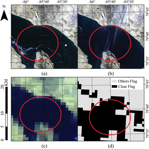
Figure 2. Spatial distribution of selected AERONET stations over the BTH region. The background image is the Terra and Aqua combined MODIS land cover type (MCD12Q1) Version 6. The colours in this figure legend represent different land cover types and the land cover types are evergreen needleleaf Forests(1), evergreen Broadleaf Forests(2), deciduous needleleaf Forests(3), deciduous Broadleaf Forests(4), mixed Forests(5), closed Shrublands(6), open Shrublands(7), Woody Savannas(8), Savannas(9), Grasslands(10), permanent wetlands (11), Croplands(12), urban and Built-up Lands(13), Cropland/Natural vegetation Mosaics(14), permanent snow and ice (15), Barren(16), and water Bodies(17) respectively.
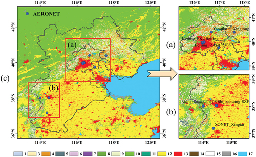
Table 1. Detailed information about the used AERONET sites. Lat: latitude; Lon: longitude.
Table 2. Detailed information of MODIS/Terra data used in this study.
Table 3. Performance of AOD retrievals under different sub-region sizes. In the collection 6 AOD validation, EE is defined as ±0.05 or ±0.15×AOD, and the AERONET site coverage represents effective coverage of AERONET AOD for the period 2011–2020.
Figure 3. The pipeline of the SPAODnet algorithm.
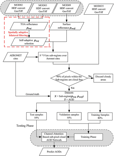
Figure 4. The visualization results of bilateral filtering in removing sub-pixel pixels. (a) and (b) show sentinel 2 satellite images under clear and cloudy conditions, respectively. (c) shows a low-resolution MODIS image under cloudy conditions. (d) demonstrates the results of Gaussian filtering, thresholding, and bilateral filtering in removing sub-pixel clouds from MODIS images.
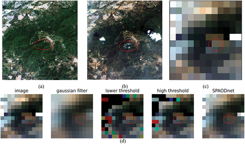
Figure 5. A schematic representation of the channel-attention-based convolutional neural network architecture used to retrieve AOD. The same architecture was optimized multiple times with different loss functions to compare the sensitivity of the model. Convolution, channel attention, average pooling, up-sampling plus channel attention, global pooling, dense, and dropout layers are shown in purple, white, blue, green, blue, pink, and sky blue respectively. The concatenated denotes the concatenation operation between feature maps.
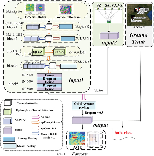
Figure 6. Diagram of the Up-CA module. As illustrated, this module utilizes 1*1 convolutional layer instead of global pooling. The green and yellow blocks represent the depthwise separable convolution for conv 3*3 and conv1*1 respectively. ⊙ represents the sigmoid function. ⊙ is the matrix dot product. ⊗ denotes matrix multiplication. Convolution kernel size is 3*3 and the stride is 1 in convolution operation.
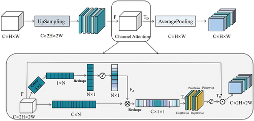
Figure 7. Comparison of the performance of AOD retrieval on SPAODnet using different loss functions.
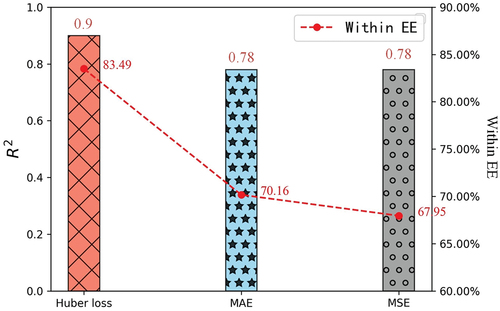
Figure 8. (a-c) the daily MODIS TOA reflectance true color maps over the BTH in China with 0.5 km resolution on 2,019,072; 2019267 and 2,020,158 respectively. (d-f) the daily maps of AOD retrieval as derived over the BTH in China using the SPAODnet model applied to MODIS-Aqua data at 0.550 μm with 1 km resolution. (g-I) the daily maps of AOD retrieval using the deep blue algorithm and deep target algorithm applied to MODIS-Aqua with a resolution of 10 km and 3 km, respectively. (m-r) the daily maps of AOD retrieval using the deep learning model NNero and MAIAC with 1 km resolution. The spatial distribution of AERONET site is represented by yellow triangles the white area in the maps represents no data.
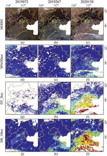
Figure 8. (Continued).
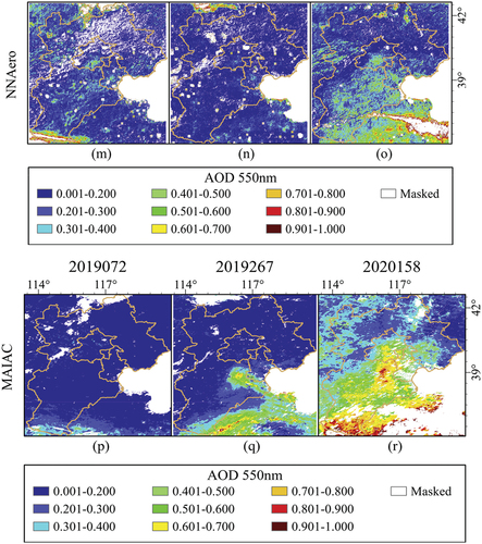
Table 4. Test performances for the AODs from the MAIAC, SPAODnet, MODIS DB products, and the major AERONET sites. QA = 1, 2, and 3 represent the quality assurance levels of DB products.
Figure 9. Density scatterplots of total samples for (a) the MAIAC algorithm, (b) the deep blue algorithm, (c) the dark target algorithm, (d) the deep blue algorithm and the dark target algorithm (DBDT) and (e) SPAODnet algorithm. The colour bars represent the density of retrieved values that rely on the grid points (his2D). The black solid line is the 1:1 line, and the red dashed lines represent the within EE lines.
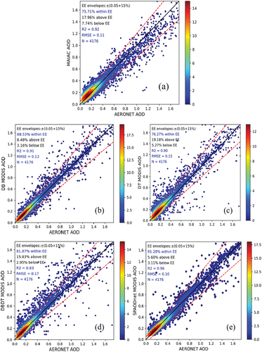
Figure 10. Scatter plots with independent test for the retrieval of AOD. (a) the MAIAC algorithm, (b) the deep blue algorithm, (c) the dark target algorithm, (d) the deep blue algorithm and the dark target algorithm (DBDT) and (e) the SPAODnet algorithm.
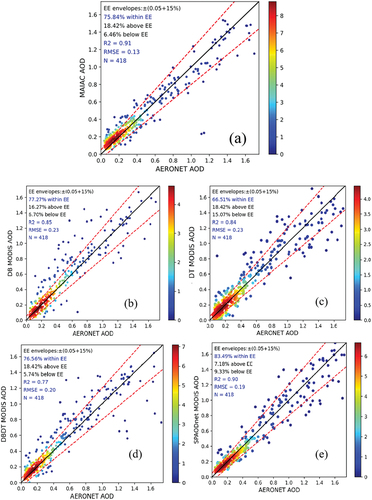
Figure 11. Performance comparison between the (a) NNAero model and (b) SPAODnet model.
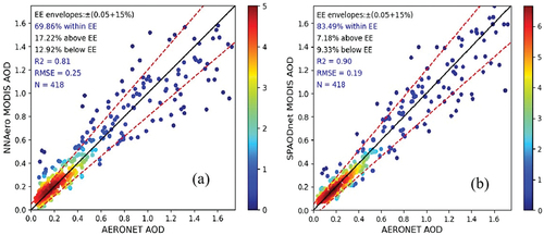
Figure 12. The histogram of the retrievable number and the AOD site coverage from DB algorithm and SPAODnet in the BTH region during 2011–2020. (a) reveal the number of retrievable aerosols. (b) reveal the corresponding AOD site coverage.
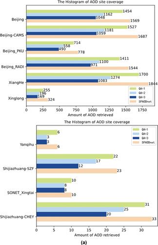
Figure 12. (Continued).
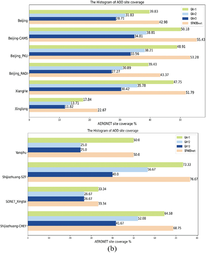
Figure 13. The daily of MODIS TOA reflectance true colour maps and the attention maps derived from Grad-CAM. A lighter colour indicates a higher weight and yellow indicates the highest weight.
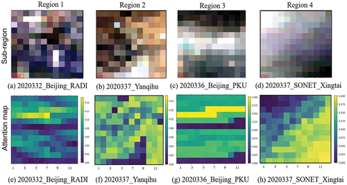
Table 5. The ablation experiment of SPAODnet.“above EE” is the metric used to quantify sub-pixel clouds.
Data availability statement
The data that support the findings of this study are available upon request by contact with the corresponding author, or accessed through https://ladsweb.modaps.eosdis.nasa.gov/and https://aeronet.gsfc.nasa.gov/cgi-bin/webtool_aod_v3.