Simulating urban growth by coupling macro-processes and micro-dynamics: a case study on Wuhan, China

Figures & data

Figure 1. Geographic location of the study area (Wuhan, Hubei Province, China).

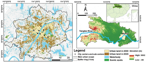
Figure 2. Framework of the proposed urban growth model.

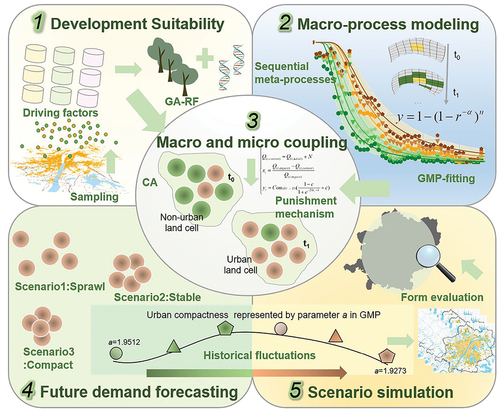
Figure 3. Conceptual diagram of the geographic micro-process (GMP) model developed in this study. (a) portrays the accumulation of geographic meta-processes, and (b) portrays the influence of parameter regulation.

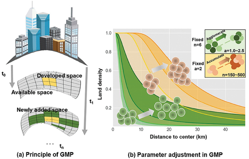
Figure 4. Illustration of the geographic micro-process (GMP) model used in this study. (a) GMP-fitting results; (b) portrays the variations in the$\alpha$ parameter. The graphical shapes represent different time nodes. (c) increment proportion of land cells in each buffer ring. Green-based color denotes the data for 1995–2005, yellow-based color denotes the data for 2010–2020.

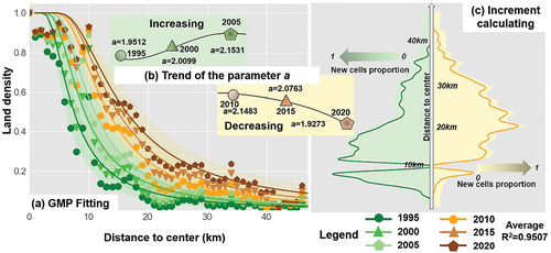
Table 1. Geographic micro-process (GMP)-fitting results and calculated cell number in different scenarios.

Year	Cells number	$\alpha$	n	R^2
1995	342969	1.9512	35.5309	0.9527
2000	457734	2.0099	61.6351	0.9320
2005	566709	2.1531	178.7755	0.9346
2010	774160	2.1483	180.0099	0.9529
2015	939769	2.0763	190.0693	0.9657
2020	1089207	1.9273	151.2663	0.9661

Figure 5. Comparison of simulation results and demand intensity of each buffer for 2020. (a–c) simulation results of non- geographic micro-process (GMP)-based model, true situation, and GMP-based models respectively. (d) graph portraying the standardized distribution of the newly-born cells.

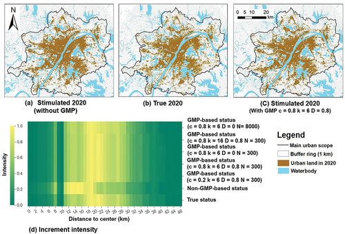
Figure 6. Fitting diagram of the penalty term and the accuracy evaluation results of each model. (a) penalty-fitting results; (b) Kappa value results; (c) figure-of-merit (FoM) index results; (d) morphological similarity (MS) index results; geographic micro-process (GMP).

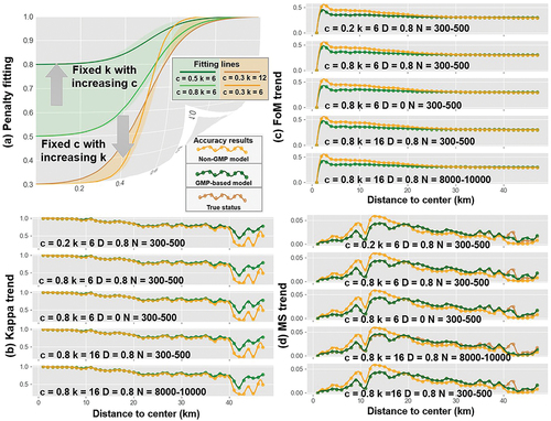
Figure 7. Simulations for various scenarios for 2025 and geographic micro-process (GMP)-fitting results. (a–c) results for compact, stable, and sprawl development, respectively; (d) GMP-fitting results for various scenarios for 2025 and 2030.

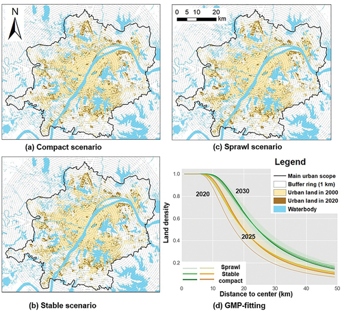
Figure 8. Simulation of various scenarios for 2030 and Grey model fitting results. (a–c) results for compact, stable, and sprawl development, respectively; (d) graph portraying the accuracy of the gray prediction algorithm.

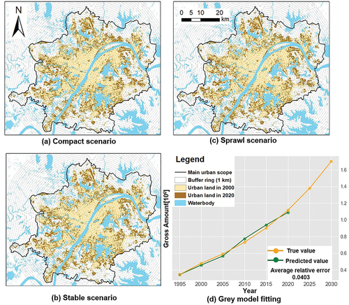
Table 2. Geographic micro-process (GMP)-fitting results and calculated cell number for different scenarios.

Year	Cells number	Scenario	$\alpha$	n
2025	1377634	Compact	2.1531	441.0967
		Sprawl	1.9273	219.5153
		Stable	2.0444	315.2021
2030	1701490	Compact	2.1531	675.9306
		Sprawl	1.9273	331.3155
		Stable	2.0444	479.4774

Table 3. Evaluation results for different scenarios.

Year	Scenario	Type of indicator
		Concentration			Connectivity		Exchange
		R^0.75（km）	R^0.25（km）	UCI	AD（km）	AD/SD	R（km）	N	SO
2025	Compact	14.5438	30.1729	0.482	16.0011	0.7115	17.669	694854	0.6379
	Sprawl	13.8676	31.3177	0.4428	16.172	0.7191	17.669	677587	0.6221
	Stable	14.2321	30.6876	0.4638	16.3622	0.7276	17.669	686787	0.6305
2030	Compact	17.7281	36.7864	0.4819	12.7113	0.5652	19.7007	922399	0.6812
	Sprawl	17.1602	38.7704	0.4426	12.9104	0.5741	19.7007	904470	0.668
	Stable	17.4672	37.6742	0.4636	12.8081	0.5695	19.7007	914008	0.675

Figure 9. Effects of each parameter of the penalty term: (a–d) effects of the c, k, D, and N parameters on the experimental results, respectively; geographic micro-process (GMP).

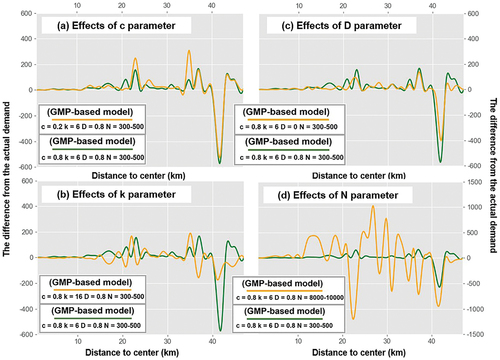
Table 4. Comparison of precision changes of different combinations of c, k, D, and N parameters.

Type of model					Kappa	FoM	MS
Non-GMP-based CA					0.8389	0.2862	0.01402
GMP-based CA (no punishment)					0.8459	0.2998	0.01382
GMP-based CA	c = 0.2	k = 6	D = 0.8	N = 300–1000	0.8516	0.3024	0.01340
	c = 0.8	k = 6	D = 0.8	N = 300–1000	0.8518	0.3024	0.01338
	c = 0.8	k = 6	D = 0	N = 300–1000	0.8516	0.3019	0.01337
	c = 0.8	k = 16	D = 0.8	N = 300–1000	0.8516	0.3018	0.01337
	c = 0.8	k = 6	D = 0	N = 8000–10000	0.8519	0.3034	0.01341

*MS of the true scenario is 0.01336.

Data availability statement

The data that support the findings of this study are available from the first author upon reasonable request.