D-FusionNet: road extraction from remote sensing images using dilated convolutional block

Figures & data

Figure 1. The GF-2 dataset (a to j represent data from the GF-2 dataset. We used white color to depict the annotated road areas by overlaying road labels onto image tiles).

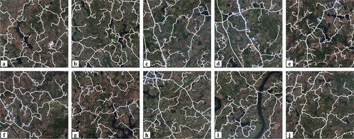
Table 1. The parameters of GF-2 images used in this study.

Time	Centre	Resolution (m)	Orbit Number	Sensor	Cloud Cover (%)
2021.09.20	N29.20, E105.39	3.24	38317	PMS2	0
2020.04.15	N29.18, E105.42	3.24	30575	PMS2	0
2018.03.09	N29.17, E105.35	3.24	19209	PMS2	0

Figure 2. Dilated convolutional block (the green square represents the learning region of dilated convolution, the white square represents the “hole” of dilated convolution, which refers to the gaps between the convolutional units. The blue shadows at the bottom of the figure depict the receptive field).

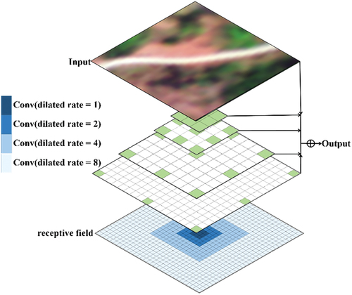
Figure 3. Structure of D-FusionNet. (The encoder-decoder in this figure is composed of different modules, represented by the rectangular blocks of various colors. The dashed lines indicate the specific operations performed by each block, while the solid lines represent the connections within the network. The rectangles of different colors correspond to the various standard operations in CNNs, and the group of gray rectangles represents the current feature map).

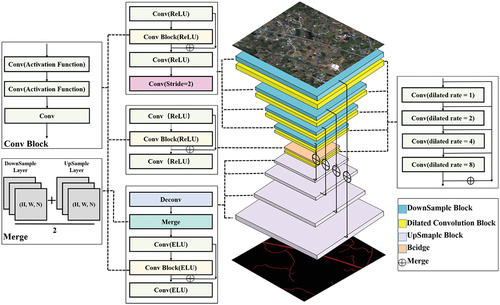
Figure 4. The flowchart of the experimental process (The sources of a-1 and b-1 are the Massachusetts dataset and the GF-2 dataset, respectively. The extraction results can be seen in a-2 and b-2. c demonstrates the Spatial transferability of D-FusionNet).

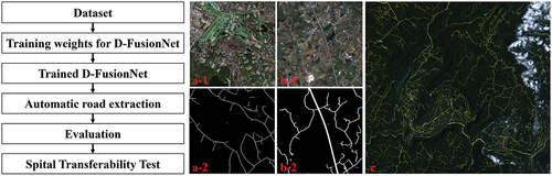
Figure 5. Grad-CAM analysis of ablation models in dilation rate experiment (ablation I, II, III, IV and V represents the ablation model by replacing the dilation rate in DCB with {2, 4, 8, 16}, {4,8,16,32}{32,16,8,4}{16,8,4,2}{8,4,2,1}, respectively).

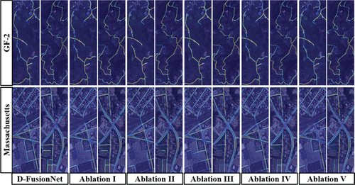
Table 2. Ablation experiments by modifying the dilation rates.

DCB		Dataset		F1-Score (%)	IoU (%)	MCC (%)
Dilation Rate	Position	GF-2	MASSACHUSETTS
{1,2,4,8}	{1,2,3,4,5}	√		81.70	69.05	80.77
			√	78.11	64.08	77.88
{2,4,8,16}	{1,2,3,4,5}	√		81.31 ↓0.39	68.51 ↓0.54	80.38 ↓0.39
			√	77.82 ↓0.29	63.70 ↓0.38	77.76 ↓0.12
{4,8,16,32}	{1,2,3,4,5}	√		80.99 ↓0.71	68.05 ↓1.00	80.02 ↓0.75
			√	77.14 ↓0.97	62.78 ↓1.3	77.19 ↓0.69
{32,16,8,4}	{1,2,3,4,5}	√		80.79 ↓0.91	67.78 ↓1.27	79.82 ↓0.95
			√	77.55 ↓0.56	63.33 ↓0.75	77.44 ↓0.44
{16,8,4,2}	{1,2,3,4,5}	√		80.34 ↓1.36	67.14 ↓1.91	79.34 ↓1.43
			√	77.73 ↓0.38	63.58 ↓0.5	77.41 ↓0.47
{8,4,2,1}	{1,2,3,4,5}	√		81.44 ↓0.26	68.69 ↓0.36	80.50 ↓0.27
			√	77.43 ↓0.68	63.17 ↓0.91	77.33 ↓0.55

D-FusionNet's accuracy and the maximum differences observed on different datasets are highlighted in bold

Figure 6. The Grad-CAM analysis of ablation models in embedding positions experiment. Ablation I, II, III, IV, and V represent the ablation model by removing the downsampling performed after the first, second, third, fourth, and fifth iteration.

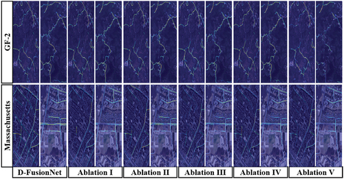
Table 3. Ablation experiments by modifying the embedding positions.

DCB		Dataset		F1-Score (%)	IoU (%)	MCC (%)
Dilation Rate	Position	GF-2	MASSACHUSETTS
{1,2,4,8}	{1,2,3,4,5}	√		81.70	69.05	80.77
			√	78.11	64.08	77.88
{1,2,4,8}	{2,3,4,5}	√		81.11 ↓0.59	68.21 ↓0.84	80.19 ↓0.58
			√	77.56 ↓0.55	63.34 ↓0.74	77.79 ↓0.09
{1,2,4,8}	{1,3,4,5}	√		81.28 ↓0.42	68.46 ↓0.59	80.34 ↓0.43
			√	77.21 ↓0.9	62.88 ↓1.20	77.15 ↓0.73
{1,2,4,8}	{1,2,4,5}	√		81.09 ↓0.61	68.19 ↓0.86	80.13 ↓0.64
			√	77.86 ↓0.25	63.74 ↓0.34	77.72 ↓0.16
{1,2,4,8}	{1,2,3,5}	√		81.37 ↓0.33	68.60 ↓0.45	80.43 ↓0.34
			√	77.24 ↓0.87	62.92 ↓1.16	77.49 ↓0.39
{1,2,4,8}	{1,2,3,4}	√		81.54 ↓0.16	68.84 ↓0.21	80.60 ↓0.17
			√	77.55 ↓0.56	63.33 ↓0.75	77.40 ↓0.48

D-FusionNet's accuracy and the maximum differences observed on different datasets are highlighted in bold

Table 4. Comparisons among FCN, UNet, LinkNet, D-LinkNet, FusionNet, and proposed D-FusionNet models.

MODEL	Dataset		F1-Score (%)	IoU (%)	MCC (%)
	GF-2	MASSACHUSETTS
FCN	√		70.15 ↑11.55	54.02 ↑15.03	68.69 ↑12.08
		√	74.87 ↑3.24	59.83 ↑4.25	74.94 ↑2.94
UNet	√		80.65 ↑1.05	67.57 ↑1.48	79.66 ↑1.11
		√	76.52 ↑1.59	61.97 ↑2.11	76.59 ↑1.29
LinkNet	√		73.46 ↑8.24	58.05 ↑11.00	72.13 ↑8.64
		√	73.34 ↑4.77	57.91 ↑6.17	73.18 ↑4.70
D-LinkNet	√		76.45 ↑5.25	61.88 ↑7.17	75.25 ↑5.52
		√	75.80 ↑2.31	61.03 ↑3.05	75.74 ↑2.14
FusionNet	√		81.04 ↑0.66	68.12 ↑0.93	80.09 ↑0.68
		√	77.60 ↑0.51	63.40 ↑0.68	77.72 ↑0.16
Ours	√		81.70	69.05	80.77
		√	78.11	64.08	77.88

D-FusionNet's accuracy and the maximum differences observed on different datasets are highlighted in bold

Figure 7. The comparisons of road extraction among FCN, UNet and D-FusionNet models (for each model, the left shows the extracted road and the right shows the evaluation parameters: TP with green, FN with red, TN with black, and FP with blue. The red rectangles highlight the comparisons among FCN, UNet and D-FusionNet models).

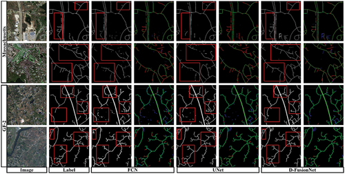
Figure 8. The comparisons of road extraction among LinkNet, D-LinkNet and D-FusionNet models (for each model, the left shows the extracted road and the right shows the evaluation parameters: TP with green, FN with red, TN with black, and FP with blue. The red rectangles highlight the comparisons among LinkNet, D-LinkNet and D-FusionNet models).

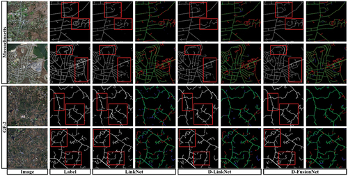
Figure 9. The comparisons of road extraction between FusionNet and D-FusionNet models (For the each model, the left shows the extracted road and the right shows the evaluation parameters: TP with green, FN with red, TN with black, and FP with blue. The yellow rectangles highlight the comparisons among LinkNet, D-LinkNet and D-FusionNet).

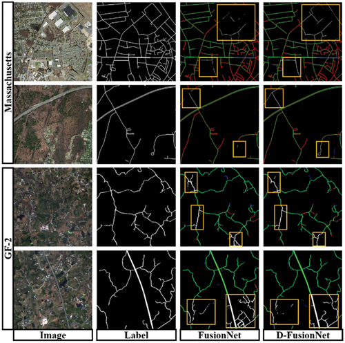
Figure 10. The roads that the D-FusionNet is difficult to extract.

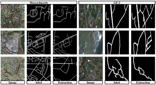
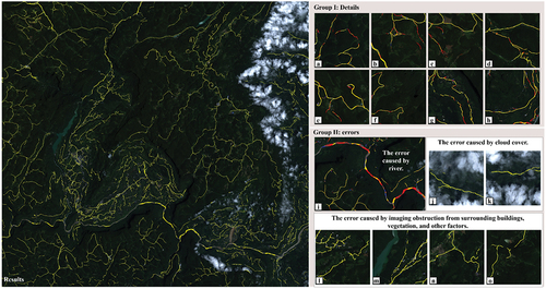
Figure 11. Spatial transferability test of D-FusionNet (The figure consists of three parts: on the left is the extraction result of D-FusionNet in the summer imagery of Enshi Tujia and Miao Autonomous Prefecture, Hubei Province. The extracted road areas are highlighted in yellow. In group I, we randomly selected eight image tiles from the imagery and compared the extraction results of D-FusionNet and FusionNet. Yellow represents the common areas extracted by both networks, red indicates the additional road areas extracted by D-FusionNet compared to FusionNet, and the meaning of blue is opposite to that of red. In group II, we demonstrate several error sources of D-FusionNet. Among them, i shows the influence of rivers on network extraction, using the same annotation method as group I. j and k demonstrate the impact of cloud and fog cover on network extraction. l~o illustrate the impact of imaging obstruction from surrounding buildings, vegetation, and other factors on network extraction. The annotation method for j~o is the same as that on the left side of the figure).

Data availability statement

The public dataset used in this study can be obtained from https://www.cs.toronto.edu/~vmnih/data/. The satellite imagery data involved in the study can be acquired from the China Center for Resources Satellite Data and Application at https://www.cresda.com/zgzywxyyzx/index.html.