Diagnosing urban traffic anomalies by integrating geographic knowledge and tensor theory

Figures & data

Figure 1. Tensor construction and transformation.

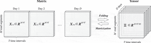
Figure 2. Overview of urban anomaly detection and analysis framework.

Figure 3. Urban adjacent road topology. Central road a is adjacent to roads B1–B6 in the first order and roads C1–C15 roads in the second order.

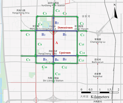
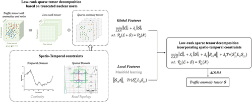
Figure 4. Specific ST-LRST procedure.

Table

Algorithm 1 Solving ST-LRST for Urban Anomaly Detection

Input: Traffic speed tensor $\mathcal{X}\in {\mathbb{R}}^{M\times N\times T}$; decomposed matrices A, B; penalty parameters ρk, α, β, γ, φ; weight parameters pk, λk (k = 1,2,3); anomaly spatiotemporal correlation matrices Δ, LA. Initialize: ${\mathcal{P}}_{\mathrm{\Omega }}({\mathcal{L}}_k^0)={\mathcal{P}}_{\mathrm{\Omega }}({\mathcal{M}}^0)={\mathcal{P}}_{\mathrm{\Omega }}(\mathcal{X})$, ${\mathcal{S}}^0={\mathcal{W}}^0={\mathcal{Z}}^0={\mathcal{V}}^0={\mathcal{T}}_k^0={\mathcal{Y}}_d^0=0\in {\mathbb{R}}^{M\times N\times T}$, (k = 1,2,3; d = 1,2,3,4); δ, ${\rho }_k^{max}$, α^max, β^max, γ^max, φ^max, ɛ, MaxIter. Iter = 0; While Iter ≤ MaxIter and not converged do Update penalty parameters using Eq. (A.18) in Appendix A; For k = 1 to 3 do Update tensors $\mathcal{L}$k via Eq. (A.5); End For Update sparse tensor $\mathcal{S}$ via Eq. (A.8); Update auxiliary tensor $\mathcal{W}$ via Eq. (A.10); Updating temporal feature tensor $\mathcal{Z}$ via Eq. (A.12); Updating spatial feature tensor $\mathcal{V}$ via Eq. (A.14); Update auxiliary tensor $\mathcal{M}$ via Eq. (A.16); Update dual variables via Eq. (A.17); Iter = Iter + 1; End While Output: Urban traffic anomaly tensor $\mathcal{S}$.

Table 1. Analysis of abnormal traffic status on urban roads.

Traffic Status		Event Type	Characteristics of changes	Duration	Scope of Impact	Prior knowledge
Traffic flow changes	Citywide road network	Citywide large-impact events (e.g. Olympic Games, large festivals, etc.)	Traffic increases on the whole road network	Day	Citywide	Date, POIs
		Extreme weather (typhoons, snowstorms, etc.)	Traffic reduction for the whole road network	Day	Citywide	Weather forecast
	Some road segments	Serious traffic accidents	Congestion in some areas and during some hours	Hour	Road segments	/
		Sports games and concerts	Congestion in some areas and during some hours	Hour	Road segments	Social Media, POIs
Topology changes		Road openings and closures (e.g. marathon)	Traffic status on some roads changes to 0	Hour	Road segments	Government announcement

Figure 5. The urban road network in Xi’an, China. Brown lines indicate the major road segments in the study area.

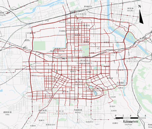
Table 2. Datasets used in this study.

Date	Duration	Resolution	Size (Matrix)	Size (Tensor)	Remarks
Apr. 2018	30 days	10min	500 × 4320	500 × 144 × 30	Simulation study, traffic flow change detection
Oct. 2018	31 days	10min	500 × 4464	500 × 144 × 31	Topology change detection

Table 3. Anomalies simulated at different scales.

Type	Impact scope (Spatial)	Impact scope (Temporal)	Impact intensity	Frequency
Anomaly #1	1st order	1 h	65%	3 times a day
Anomaly #2	2nd order	3 h	55%	once a day
Anomaly #3	3rd order	12 h	40%	once every 10 days

Table 4. Road segment traffic operation status classification.

Traffic condition	Smooth	Basically smooth	Mild congestion	Moderate congestion	Serious congestion
r	r > 70%	50% < r ≤ 70%	40% < r ≤ 50%	30% < r ≤ 40%	r ≤ 30%

Table 5. Description of different baseline models.

Data Structure		Method	Description
Vector		Isolation Forest (Liu, Ting, and Zhou 2012)	A fast outlier detection method based on Ensemble. A binomial search tree structure called isolation tree is used to perform anomaly detection for the traffic status of each road segment.
Matrix (Road segments, time intervals × days)		LRSD (TNN) (Xue et al. 2019)	A low-rank and sparse matrix decomposition method with the introduction of the truncated nuclear norm and sparse regularization for constraints.
		Improved RPCA (Wang et al. 2018)	An improved robust principal component analysis model that considers the temporal dependence of urban anomalies.
Tensor (Road segments, time-intervals, days)	Based on tensor decomposition	BATF (Chen et al. 2019)	A fully Bayesian model built on a special tensor factorization formulation that learns variables via variational Bayes.
	Based on nuclear norm relaxation	LATC (Chen et al. 2022)	A low-rank autoregressive tensor model that introduces truncated nuclear norm and temporal variation to effectively characterize both global patterns and local consistency in spatiotemporal traffic data.
		TRPCA (NN) (Hu and Work 2021)	Also named LRST, a tensor robust principal component analysis method that uses nuclear norm as a convex substitution of the rank function to extract low-rank tensors.
		TRPCA (t-SVT) (Lu et al. 2020)	A tensor robust principal component analysis method with a new tensor nuclear norm that uses tensor Singular Value Threshold (t-SVT) as the proximity operator associated with the tensor nuclear norm.

Table 6. Performance comparison for single-type anomaly detection. Bold values indicate the best performance among the considered models.

Scenario	Criterion	Isolation Forest	LRSD	Improved PRCA	BATF	LATC	TRPCA (NN)	TRPCA (t-SVT)	ST-LRST (Ours)
Anomaly #1	Precision	81.56%	87.18%	99.66%	81.55%	87.03%	100.00%	98.18%	100.00%
	Recall	60.03%	100.00%	96.85%	100.00%	100.00%	99.75%	100.00%	99.88%
	F1-Score	69.16%	93.15%	98.23%	89.84%	93.07%	99.88%	99.08%	99.94%
Anomaly #2	Precision	100.00%	75.77%	68.43%	67.63%	71.52%	83.76%	87.49%	97.46%
	Recall	40.65%	72.55%	100.00%	98.02%	100.00%	100.00%	100.00%	100.00%
	F1-Score	57.81%	74.13%	81.26%	80.03%	83.40%	91.16%	93.33%	98.71%
Anomaly #3	Precision	98.93%	61.61%	59.90%	28.19%	64.58%	78.21%	82.25%	96.76%
	Recall	20.56%	18.03%	100.00%	29.05%	75.60%	99.99%	100.00%	99.96%
	F1-Score	34.04%	27.90%	74.92%	28.61%	69.66%	87.77%	90.26%	98.33%

Table 7. Performance comparison for mixed-type anomaly detection. Bold values indicate the best performance among different models.

Model	Scope detection			Intensity analysis
	Precision	Recall	F1-Score	Accuracy	RMSE (km/h)	MAPE
Isolation Forest	67.00%	63.12%	65.00%	14.63%	8.31	34.76%
LRSD	91.36%	64.48%	75.60%	86.18%	3.16	7.26%
Improved PRCA	84.22%	99.31%	91.14%	93.50%	1.00	5.22%
BATF	69.23%	87.82%	77.42%	80.49%	3.14	9.85%
LATC	84.84%	92.41%	88.47%	84.55%	1.56	8.85%
TRPCA (NN)	89.68%	88.06%	88.86%	92.68%	1.17	4.16%
TRPCA (t-SVT)	93.44%	92.33%	92.88%	91.06%	1.37	4.06%
LRST-TNN (ours)	86.04%	99.50%	92.28%	95.12%	0.93	4.65%
ST-LRST (ours)	97.29%	99.74%	98.50%	95.93%	0.59	3.09%

Figure 6. Daily pattern extraction results before and after the introduction of nonconvex functions. (a) road 1; (b) road 125. Blue shaded areas indicate injected anomalies.

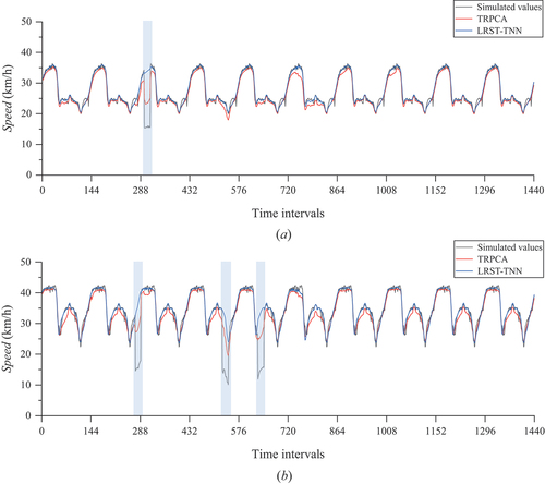
Table 8. Impact of spatial and temporal constraints on anomaly detection accuracy. Bold values indicate the best performance among different models.

Criterion	LRST-TNN	LRST-TNN + T	LRST-TNN + S	LRST-TNN + ST
Precision	86.04%	94.27%	89.09%	97.29%
Recall	99.50%	97.90%	99.56%	99.74%
F1-Score	92.28%	96.05%	94.04%	98.50%
Accuracy	95.12%	95.12%	94.31%	95.93%
RMSE (km/h)	0.93	0.76	1.10	0.59
MAPE	4.65%	3.54%	5.59%	3.09%

Figure 7. Anomaly detection results of different models. (a) road 1; (b) road 125.

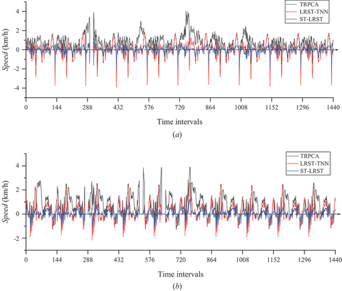
Figure 8. Effect of the introduction of spatio-temporal constraints on anomaly detection results. (a) time-192, without anomalies; (b) time-769, with anomalies. |Vc| indicates the change in speed due to anomalies.

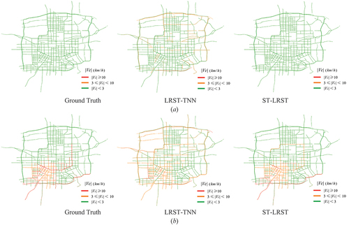
Figure 9. Anomaly detection map of urban roads in Xi’an on Tomb Sweeping Festival 2018. (a) 10:00 a.M. (b) 2:00 p.M. (c) 6:00 p.M. (d) 10:00 p.M. vc indicates the value of speed change due to anomalies.

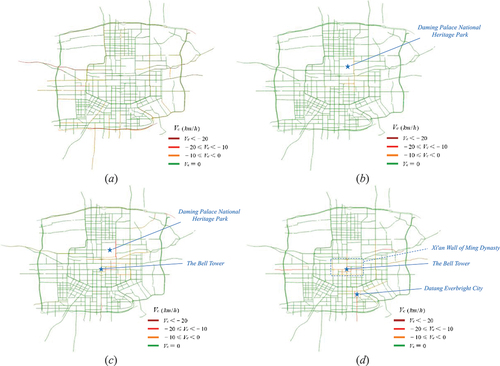
Figure 10. Map of road closures detected for the 2018 Xi’an International marathon. (a) schematic diagram of the race route, with red solid lines indicating the race roads and dashed lines indicating low-grade roads. (b) 7:30 a.M. (c) 8:30 a.M. (d) 9:30 a.M. (e) 10:30 a.M. (f) 11:30 a.M.

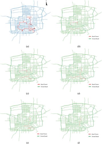
Figure 11. Map of detected road anomalies for the 2018 Xi’an International marathon. (a) 7:30 a.M. (b) 8:30 a.M. (c) 9:30 a.M. (d) 10:30 a.M. (e) 11:30 a.M. (f) 12:30 a.M. Marathon routes are shaded in blue.

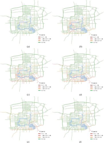
Table A1. Updated variables and related parameters.

Variables	$\mathcal{L}$k	$\mathcal{W}$	$\mathcal{Z}$	$\mathcal{V}$	$\mathcal{M}$	$\mathcal{S}$
Related parameters	pk, ρk	β, γ	λ2, γ	λ3, φ	ρk, α	λ1, α, β, φ

Figure A1. Model accuracy under different parameter settings, with axes to the power of 10.

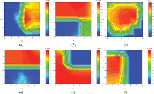
Table A2. Parameter settings of ST-LRST model.

Parameters	weight parameters				penalty parameters
	pk	λ1	λ2	λ3	ρk	α	β	γ	φ
Value	10^1	10^−2	10^−1	10^−3	10^−3	10^−3	10^−3	10^−1	10^−5

Liu, F. T., K. M. Ting, and Z.-H. Zhou. 2012. “Isolation-Based Anomaly Detection.” ACM Transactions on Knowledge Discovery from Data (TKDD) 6 (1): 1–39. https://doi.org/10.1145/2133360.2133363.

 Web of Science ®Google Scholar

Xue, Z., J. Dong, Y. Zhao, C. Liu, and R. Chellali. 2019. “Low-Rank and Sparse Matrix Decomposition via the Truncated Nuclear Norm and a Sparse Regularizer.” The Visual Computer 35 (11): 1549–1566. https://doi.org/10.1007/s00371-018-1555-1.

 Web of Science ®Google Scholar

Wang, X., Y. Zhang, H. Liu, Y. Wang, L. Wang, and B. Yin. 2018. “An Improved Robust Principal Component Analysis Model for Anomalies Detection of Subway Passenger Flow.” Journal of Advanced Transportation, 2018 2018:1–12. https://doi.org/10.1155/2018/7191549.

 Google Scholar

Chen, X., Z. He, Y. Chen, Y. Lu, and J. Wang. 2019. “Missing Traffic Data Imputation and Pattern Discovery with a Bayesian Augmented Tensor Factorization Model.” Transportation Research Part C: Emerging Technologies 104:66–77. https://doi.org/10.1016/j.trc.2019.03.003.

 Web of Science ®Google Scholar

Chen, X., M. Lei, N. Saunier, and L. Sun. 2022. “Low-Rank Autoregressive Tensor Completion for Spatiotemporal Traffic Data Imputation.” IEEE Transactions on Intelligent Transportation Systems 23 (8): 12301–12310. https://doi.org/10.1109/TITS.2021.3113608.

 Web of Science ®Google Scholar

Hu, Y., and D. B. Work. 2021. “Robust Tensor Recovery with Fiber Outliers for Traffic Events.” ACM Transactions on Knowledge Discovery from Data 15 (1): 1–27. https://doi.org/10.1145/3417337.

 Web of Science ®Google Scholar

Lu, C., J. Feng, Y. Chen, W. Liu, Z. Lin, and S. Yan. 2020. “Tensor Robust Principal Component Analysis with a New Tensor Nuclear Norm.” IEEE Transactions on Pattern Analysis and Machine Intelligence 42 (4): 925–938. https://doi.org/10.1109/TPAMI.2019.2891760.

 PubMed Web of Science ®Google Scholar