
Figures & data
Figure 1. The location of our study area. In the figure (c-d), the black polygons denote the administrative boundary, and the blue polygons denote the coastal expansion areas.
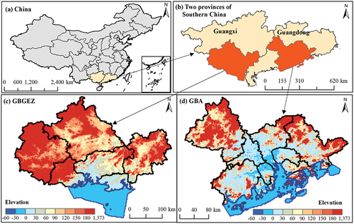
Table 1. Classification system of wetland ecosystem.
Figure 2. Image statistics of Landsat-8 time series from June 2019 to June 2021 in our study area. (a-b) are the numbers of spatial distributions of good-quality observation (pixel without could cover) in the GBGEZ and GBA, respectively. (c-d) are histograms of good-quality observations in the GBGEZ and GBA, respectively.
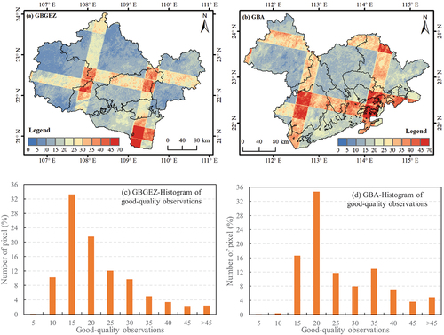
Table 2. Auxiliary dataset list in our study.
Figure 3. Workflow of detailed wetland type classification. SRTM denote Shuttle Radar Topography Mission, CECD denote China Ecosystem-type classification dataset, MC_LASAC denote HSL_MangroveChina_LASAC_share, TWEA denote tidal wetlands in East Asia.
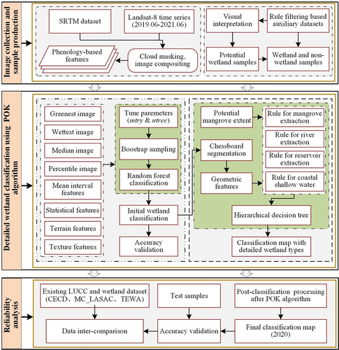
Table 3. Illustration of training sample generation based on rule filtering and visual interpretation.
Figure 4. Spatial distribution of training sample points in the GBGEZ (a) and GBA (b).
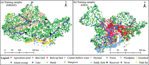
Figure 5. Concept graph of the POK algorithm. GEE denotes the Google Earth Engine. PME denote the potential mangrove extent. POK denotes the pixel- and object-based algorithm with knowledge.
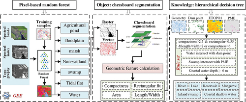
Figure 6. Phenology-based features constructed by the GEE platform.
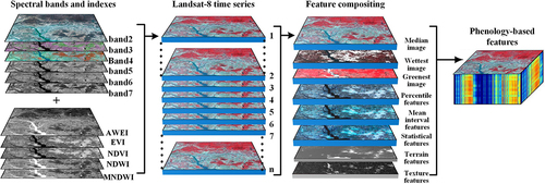
Figure 7. Geometric features of reservoirs, rivers and lakes used in the development of the rule set of hierarchical decision. The three geometric characteristics are shown for three size categories, between 0–2 km2, 2–10 km2 and 10–50 km2 for Compactness (a-c), rectangular fit (d-f) and length/width (g-i), respectively.
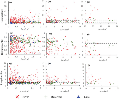
Figure 8. Illustration of hierarchical decision tree. The green boxes denote the initial input data, the yellow ovals denote process operations, the light yellow boxes denote the intermediate output, and the light blue denote the final output. In addition, it should be noted that the coastal deep water does not belong to wetlands, which was grouped into background.
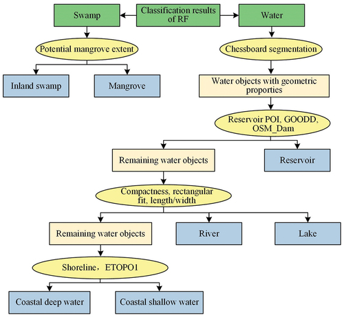
Figure 9. Spatial distribution of six wetland types and six non-wetland types.
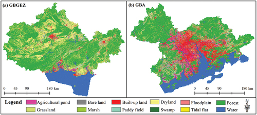
Table 4. Accuracy results of the pixel-based RF classifications.
Figure 10. Spatial distribution of 10 wetland types in 2020.
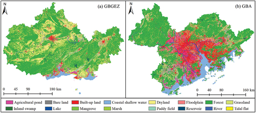
Figure 11. The spatial comparison between before and after fine classification in two typical regions. The (a) and (c) were classifications with 6 wetlands using pixel-based random forest, and the (b) and (d) were classifications with 10 wetlands using object-based hierarchical decision tree. The (a)-(b) were a typical region in GBGEZ, and the (c)-(d) are typical region in GBA.
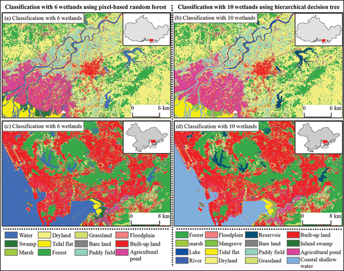
Table 5. Accuracy results of hierarchical decision tree classification.
Figure 12. Intra-comparison between our wetland maps and the CECD dataset. ourWetland refers to our wetland map.
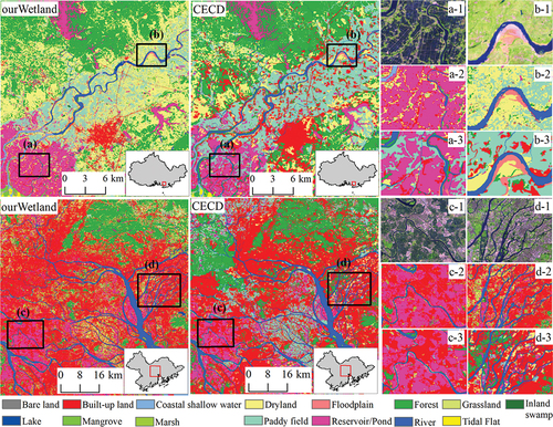
Table 6. Confusion matrix between our wetland and CECD dataset in GBGEZ. The unit is percentage (%). In this table, the diagonal values represent the percentage of consistency, while others represent the difference between two datasets.
Table 7. Confusion matrix between our wetland and CECD dataset in GBA. The unit, meanings of elements, and abbreviations are same as .
Figure 13. Intra-comparison between the MC_LASAC dataset and our mangrove. The first row shows the mangrove distribution of our wetland map in GBGEZ and GBA, respectively.
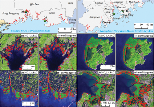
Figure 14. Intra-comparison between the TWEA dataset and our tidal flat. The first row shows the spatial distribution of the tidal flat in our wetland map.
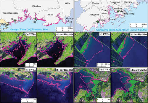
Table 8. Areas of wetland types and non-wetland types in two urban agglomerations (unit: km2).
Table A1. The corresponding relationship between the classes of CECD dataset and our wetland classification.