An investigation of inversion method to measure the radial velocity of Kuroshio from Sentinel-1 SAR data

Figures & data

Figure 1. Bathymetric map of the Kuroshio region. The solid and dashed lines represent the ascending and descending SAR data passes, respectively, the red circles are GLD buoy data, and the download link for bathymetry data: https://topex.ucsd.edu/pub/srtm15_plus/.

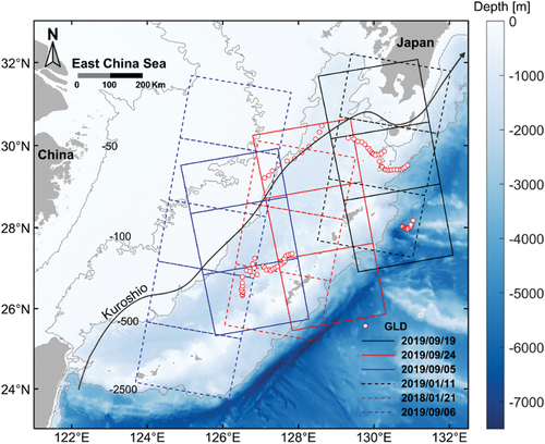
Figure 2. The flowchart of the data processing.

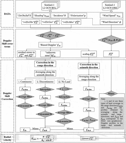
Figure 3. Three correction schemes in the range direction.

The “Note” in the manuscript is missing from the lower right corner.

Table

Range Bias Calibration Algorithm

Input: biased Doppler shit $f_{\mathrm{d}\mathrm{c}}$, landmask $Valu{e}_{Land}$, standard deviation $\delta$ Output: mean range profile $f_{dcRm}$, range profile $f_{dcR}$ $ifValu{e}_{Land}=100\mathrm{\%}continuouslandintherangedirection$ $f_{dcRm}=mean\left(f_{\mathrm{d}\mathrm{c}}\right)$ $f_{dcR}=ployfit\left(size\left(f_{\mathrm{d}\mathrm{c}}\right),2\right),filter\left(f_{dcRm}\right),3)$ $elseifValu{e}_{Land}=100\mathrm{\%}continuouslandintherangedirection$ $f_{dcRm}=fillmissing\left(mean\left(f_{\mathrm{d}\mathrm{c}}\right){,}^{\prime }media{n}^{\prime },win\right)$ $f_{dcR}=ployfit\left(size\left(f_{\mathrm{d}\mathrm{c}}\right),2\right),filter\left(f_{dcRm}\right),3)$ $elseValu{e}_{Land}=0\mathrm{\%}nolandintherangedirection$ $f_{dcRm}=fillmissing\left(mean\left(f_{\mathrm{d}\mathrm{c}}\left(\delta \le 4Hz\right)\right){,}^{\prime }media{n}^{\prime },win\right)$ $f_{dcR}=ployfit\left(size\left(f_{\mathrm{d}\mathrm{c}}\right),2\right),filter\left(f_{dcRm}\right),3)$ Note: $Valu{e}_{Land}$ is the value corresponding to the variable “rvlLandCoverage” of Sentinel-1 Level 2 OCN, 100 and 0 represent land and sea, respectively. $mean\left(f_{\mathrm{d}\mathrm{c}}\right)$ is the mean value from each column, and the pixels of each column exceed 10. $size\left(f_{\mathrm{d}\mathrm{c}}\right),2)$ and $fillmissing$ are the number of columns of the image and interpolation, respectively. As seen the histogram in Figure 3(c1,c2), Doppler shifts over land satisfies the assumption of being equal to 0 HZ.

Figure 4. Doppler shifts in the azimuth direction, with is a $\pm$10 Hz periodic variation. Figure (a) shows the identification process of the scalloping (only IW1 swath), while figure (b) shows the method applied to the full image.

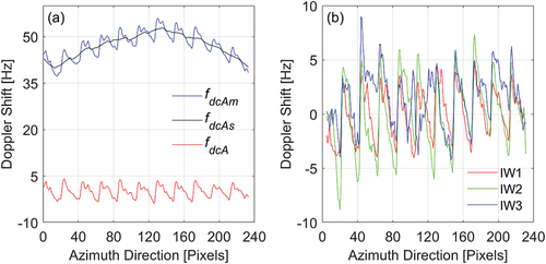
Figure 5. Result of current retrieval. Figures (a) and (b) show the radial velocities on September 24, 2019, and January 21, 2018, respectively. The Kuroshio central current is the blue line, and the Kuroshio counter Current is the red line. The arrows are derived from the MOB products.

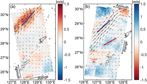
Figure 6. Comparing SAR radial surface velocity with the GLD data. Figure (a) is only the azimuth correction completed, while figure (b) shows the results of range and azimuth calibration. Figure (c) shows the results of wind-wave bias correction.

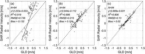
Figure 7. Comparison with ROMS model. (a) shows the ROMS model projected onto the SAR radial direction. (b) depicts a scatter, with different colors representing matching points from different swaths. (c) shows the histogram of the velocities difference (D-Value) between SAR and ROMS.

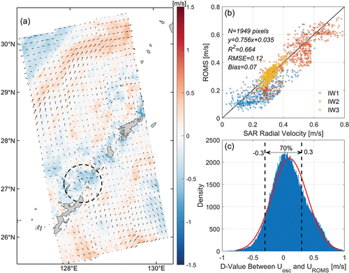
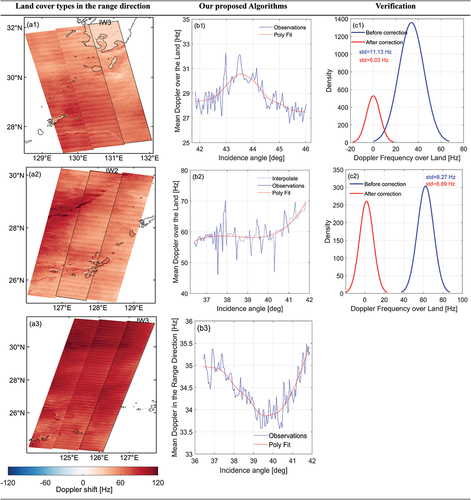
Figure 8. Non-geophysical Doppler correction. (a1) and (a2) show the biased Doppler shift $f_{\mathrm{d}\mathrm{c}}$. (b1) and (b2) show the results after correction in the range direction. (c1) and (c2) show the effective geophysical Doppler shift $f_{dc}^{phys}$ after removing the scalloping.

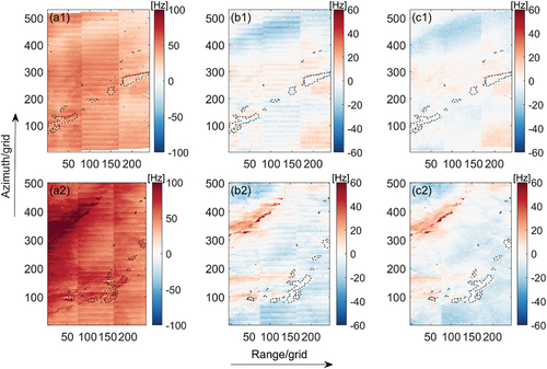
Figure 9. Non-geophysical Doppler shift variation in range direction. Figures (a) and (b) show the estimated range bias for the ascending (19 September 2019) and descending (11 January 2019), respectively. Blue line is the mean Doppler shift over land along azimuth, and red line is the error fitting value.

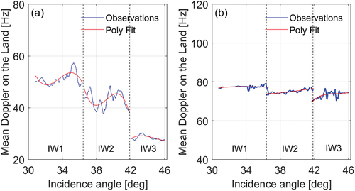
Figure 10. Comparison of three range bias estimation schemes.

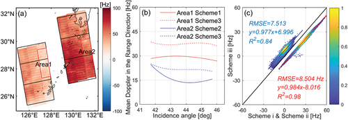
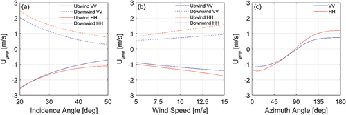
Figure 11. Variation of the Doppler velocity contributed by the ocean condition for different incidence angles, wind speeds, wind directions, and polarization parameters.

Data availability statement

The Sentinel-1 SAR OCN products that support the findings of this study are openly available at https://scihub.copernicus.eu/dhus/#/home.