Land subsidence in Beijing: response to the joint influence of the South-to-North Water Diversion Project and ecological water replenishment, observed by satellite radar interferometry

Figures & data

Table 1. Summary of relevant studies on the effects of the SNWD on land subsidence in Beijing.

Method	Datasets	Subsidence development	Reference
Modified Geodesy and Earth Observing Systems (GEOS) Advance Time Series Analysis (MATSA) and GEOS-small baseline subset (SBAS)	Advanced Land Observing Satellite-1 (ALOS-1) (2007.01–2011.0) RADARSAT-2 (2011.06–2014.12) Sentinel-1 (2014.12–2020.01)	The contribution of the SNWD is apparent since November 2016, alleviating the LS problem to a certain extent.	(Du et al. 2021)
LS monitoring stations	Monitoring station data (2004–2019)	The main contribution layer of LS shifted to strata at depth of 100 m. In addition, the stable water supply supported by the SNWD has effectively inhibited rapid LS expansion.	(Yang et al. 2021)
Stratified monitoring	Multi-depth extensometer data (2004.04–2019.04)	At present, in the Beijing LS area, the compression of shallow soil has declined, but the soil in the middle and deep parts continues to be compressed at a high speed.	(Liu et al. 2022)
Persistent Scatterer interferometric synthetic aperture radar (PS-InSAR)	RADARSAT-2 (2010.12–2014.12) Sentinel-1 (2014.12–2017.12)	InSAR results show that LS exhibits a decreasing tendency in the central portion of the North Beijing Plain.	(Zhu et al. 2020)
PS-InSAR	ENVIronmental SATtellite (ENVISAT)/Advanced SAR (ASAR) (2004.01–2010.08) RADARSAT-2 (2010.11–2014.12) Sentinel-1 (2015.06–2017.05)	After the SNWD, InSAR measurements have shown that approximately 45% of the area exhibits LS deceleration (2015–2017) relative to 2011–2014 in the Beijing Plain.	(Lyu et al. 2019)
GEOS-differential InSAR (DInSAR)	ALOS-1 Phased Array L-band SAR (PALSAR) (2007.01–2011.01) Sentinel-1 (2015.07–2016.11) ALOS-2 PALSAR (2014.09–2017.02)	Due to the SNWD, some townships in Beijing have experienced a decreasing trend in subsidence.	(Du et al. 2017)

Figure 1. Description of the study area. (a) The coverage of the synthetic aperture radar (SAR) datasets and the position of the south-to-north water diversion project middle route (SNWD-MR) are displayed in the upper left panel. The positions of the monitoring wells and levelling benchmarks are displayed in the upper right panel. (b) Lithological distribution along the Beijing section of the Yongding River (YDR) (revised after (Cao et al. 2022)). The aquifer system can be divided into zone a (single layer of sand and gravel), zone B (multiple layers of sand and gravel and a few sand layers), zone C (multiple layers of sand and a few gravel layers), and zone D (multiple layers of sand).

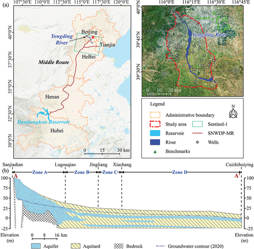
Table 2. Characteristics of the SAR images used in this study.

Sensor	Sentinel-1
	Sentinel-1A	Sentinel-1B
Band/wavelength (cm)	C/5.6
Altitude (km)	693
Path/frame	47/461
Orbit direction	Descending
Image mode	Interferometric wide swath
Polarization	Vertical–vertical
Number of images	6	54
Date range	20150617–20160611	20161003–20201111

Figure 2. The framework of the SBAS technique.

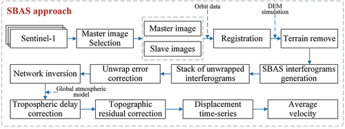
Figure 3. The SBAS network of interferograms for SAR datasets.

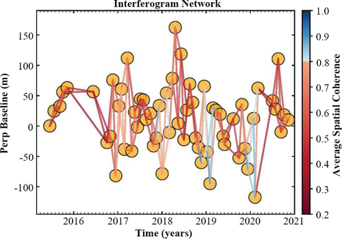
Figure 4. (a) The vertical displacement velocity map along the YDR derived from the S1A/B datasets is computed using the small baseline subset (SBAS) technique, where negative values indicate subsidence and positive values indicate uplift., (b) the histogram of the mean displacement rate., and (c) the statistics of various subsidence velocities at slowly decorrelating filtered phase (SDFP) points are presented.

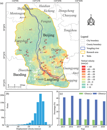
Figure 5. Accumulative time-series deformation revealed by the InSAR technique, which highlights selected points in Figure 4a, is shown.

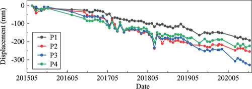
Figure 6. Cross-comparison between interferometric synthetic aperture radar (InSAR) measurements and levelling data.

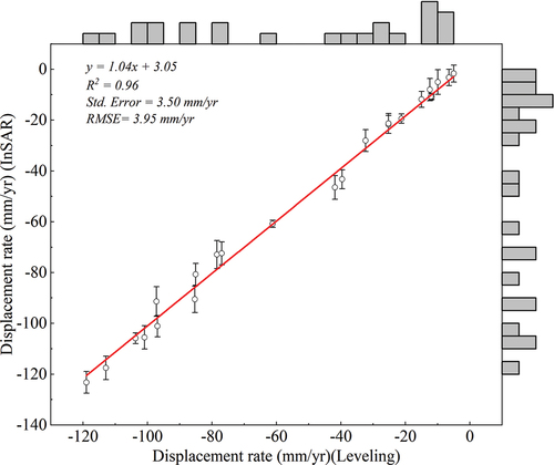
Figure 7. Annual precipitation anomalies and water resource information for the Beijing plain from 1999 to 2020.

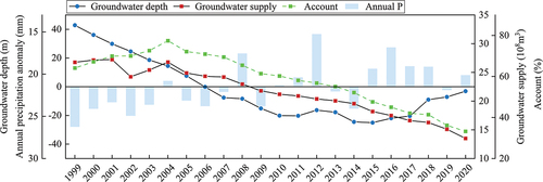
Figure 8. (a) Distribution of monthly groundwater level changes in 31 wells from 2010 to 2014 and from 2015 to 2018. (b) The change in groundwater levels in 2018 compared to 2014.

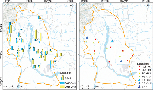
Figure 9. The nonlinear trend of time series groundwater level marked by black circles in Figure 3(a).

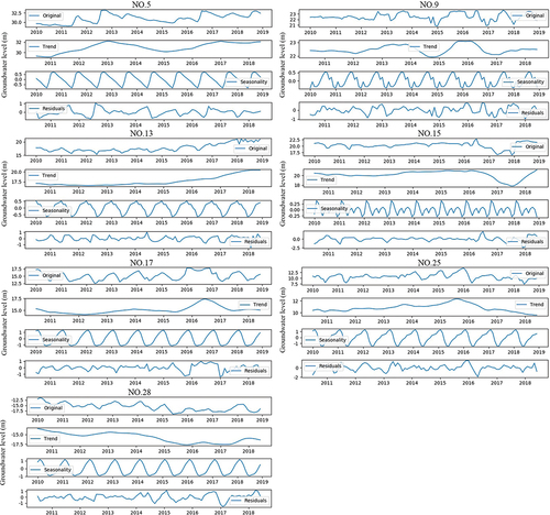
Figure 10. Profiles of the InSAR vertical subsidence time series (June 2015 to November 2020) marked by a blue dashed line in the upper left corner.

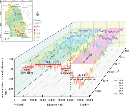
Figure 11. Annual subsidence rate along the YDR (2016–2020).

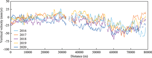
Figure 12. (a) Annual subsidence slope and (b) accumulative subsidence slope along YDR obtained from InSAR measurements (2015–2020).

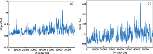
Figure 13. The groundwater level changes, and ground displacement retrieved from the InSAR technique at the monitoring wells (the locations are shown in Figure 3a).

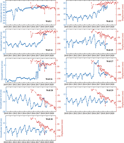
Table 3. The lag period (month) of the LS response to changes in groundwater levels in the groundwater observation wells (part).

No.	Lag Period	R^2	PDL Model
3	6	0.76	$\hat{y}=-0.02771-0.00193x_t-0.00157x_{\mathit{t}-1}-0.00125x_{\mathit{t}-2}-0.00095x_{\mathit{t}-3}-0.00067x_{\mathit{t}-4}-0.00042x_{\mathit{t}-5}-0.00020x_{\mathit{t}-6}$
25	6	0.82	$\hat{y}=0.82109+0.00490x_t+0.00272x_{\mathit{t}-1}+0.00134x_{\mathit{t}-2}+0.00075x_{\mathit{t}-3}+0.00097x_{\mathit{t}-4}+0.00199x_{\mathit{t}-5}+0.00380x_{\mathit{t}-6}$
26	4	0.70	$\hat{y}=0.00247+0.00048x_t+0.00170x_{\mathit{t}-1}-0.00307x_{\mathit{t}-2}-0.00640x_{\mathit{t}-3}-0.00087x_{\mathit{t}-4}$
30	5	0.60	$\hat{y}=-0.05326+0.01271x_t+0.00715x_{\mathit{t}-1}+0.00427x_{\mathit{t}-2}+0.00382x_{\mathit{t}-3}+0.00555x_{\mathit{t}-4}+0.00924x_{\mathit{t}-5}$

Du, Z., L. Ge, A. H.-M. Ng, X. Lian, Q. Zhu, F. G. Horgan, and Q. Zhang. 2021. “Analysis of the Impact of the South-To-North Water Diversion Project on Water Balance and Land Subsidence in Beijing, China Between 2007 and 2020.” Journal of Hydrology 603 (PB): 126990. Elsevier B.V https://doi.org/10.1016/j.jhydrol.2021.126990.

 Google Scholar

Yang, Y., H. Liu, Y. Luo, K. Lei, and X. Wang. 2021. “Development Characteristics of Land Subsidence in Eastern Beijing.” Shanghai Land & Resources 42 (1): 7–12+18. https://doi.org/10.3969/j.issn.2095-1329.2021.01.002.

 Google Scholar

Liu, H., W. Cui, Y. Luo, K. Lei, Y. Yang, F. Tian, and M. Tian. 2022. “Study on the Variation Law of Land Subsidence, Groundwater Level and Pore Water Pressure in Tianzhu, Beijing Based on Stratified Monitoring.” Geological Bulletin of China 41 (04): 692–701. https://doi.org/10.12097/j.issn.1671-2552.2022.04.013.

 Google Scholar

Zhu, L., H. Gong, Y. Chen, S. Wang, Y. Ke, G. Guo, X. Li, B. Chen, H. Wang, and P. Teatini. 2020. “Effects of Water Diversion Project on Groundwater System and Land Subsidence in Beijing, China.” Engineering Geology 276:Article 105763. https://doi.org/10.1016/j.enggeo.2020.105763.

 Web of Science ®Google Scholar

Lyu, M., Y. Ke, L. Guo, X. Li, L. Zhu, H. Gong, and C. Constantinos. 2019. “Change in Regional Land Subsidence in Beijing After South-To-North Water Diversion Project Observed Using Satellite Radar Interferometry.” GIScience & Remote Sensing (1): 140–156. Taylor & Francis https://doi.org/10.1080/15481603.2019.1676973.

 Web of Science ®Google Scholar

Du, Z., L. Ge, A. H. M. Ng, X. Li, L. Li, and J. Sequeira. 2017. “Mapping Land Subsidence Over the Eastern Beijing City Using Satellite Radar Interferometry*.” International Journal of Digital Earth 11 (1): 1–26. Taylor & Francis https://doi.org/10.1080/17538947.2017.1336651.

 Google Scholar

Cao, X., Y. Zhai, M. Li, C. Pan, F. Zheng, H. Lu, X. Xia, Y. Teng, and J. Wang. 2022. “The Suitability Assessment of Groundwater Recharge by Leakage of the Yongding River.” Hydrogeology and Engineering Geology 49(01): 20–17. https://doi.org/10.16030/j.cnki.issn.1000-3665.202107069.

 Google Scholar

Data availability statement

Upon reasonable request, the corresponding author can provide the data that support the study’s conclusions.