Quantitative assessment of the scale conversion from instantaneous to daily GPP under various sky conditions based on MODIS local overpassing time

Figures & data

Table 1. Eddy covariance tower sites from the FLUXNET 2015 Tier one dataset used in this study. 39 tower sites were selected where the incoming and diffuse incoming photosynthetic photon flux density data exist.

ID	Site name	IGBP	Lat	Long	Period	Reference
AT-Neu	Neustift	GRA	47.1167	11.3175	2002–2012	Wohlfahrt et al. (2008)
BE-Bra	Brasschaat	MF	51.3076	4.5198	2002–2014
CA-Qfo	Quebec - Eastern Boreal, Mature Black Spruce	ENF	49.6925	−74.342	2003–2010
CH-Oe1	Oensingen grassland	GRA	47.2858	7.7319	2002–2008	Ammann et al. (2009)
CH-Oe2	Oensingen crop	CRO	47.2863	7.7343	2004–2014	Dietiker et al. (2010)
CZ-BK1	Bily Kriz forest	ENF	49.5021	18.5369	2004–2008	Acosta et al. (2013)
CZ-BK2	Bily Kriz grassland	GRA	49.4944	18.5429	2004–2006
DE-Geb	Gebesee	CRO	51.1001	10.9143	2002–2014	Anthoni et al. (2004)
DE-Hai	Hainich	DBF	51.0792	10.453	2002–2012	Knohl et al. (2003)
DE-Tha	Tharandt	ENF	50.9624	13.5652	2002–2014	Grünwald and Bernhofer (2007)
DK-Sor	Soroe	DBF	55.4859	11.6446	2002–2014	Pilegaard et al. (2011)
ES-Ln2	Lanjaron-Salvage logging	OSH	36.9695	−3.4758	2009
FI-Hyy	Hyytiala	ENF	61.8474	24.2948	2002–2014	Suni et al. (2003)
FI-Lom	Lompolojankka	WET	67.9972	24.2092	2007–2009	Aurela et al. (2015))
FR-Gri	Grignon	CRO	48.8442	1.9519	2004–2013	Aurela et al. (2015)
FR-LBr	Le Bray	ENF	44.7171	−0.7693	2002–2008	Berbigier et al. (2001)
FR-Pue	Puechabon	EBF	43.7413	3.5957	2002–2014	Rambal et al. (2004)
GF-Guy	Guyaflux (French Guiana)	EBF	5.2788	−52.925	2004–2014	Bonal et al. (2008)
IT-BCi	Borgo Cioffi	CRO	40.5238	14.9574	2004–2014	Vitale et al. (2016)
IT-Col	Collelongo	DBF	41.8494	13.5881	2002–2014	Valentini et al. (1996)
IT-MBo	Monte Bondone	GRA	46.0147	11.0458	2003–2013	Marcolla et al. (2011)
IT-PT1	Parco Ticino forest	DBF	45.2009	9.061	2002–2004	Migliavacca et al. (2009)
IT-Ren	Renon	ENF	46.5869	11.4337	2002–2013	Montagnani et al. (2009)
IT-Ro2	Roccarespampani 2	DBF	42.3903	11.9209	2002–2012	Tedeschi et al. (2006)
IT-SR2	San Rossore 2	ENF	43.732	10.291	2013–2014
IT-SRo	San Rossore	ENF	43.7279	10.2844	2002–2012	Chiesi et al. (2005)
NL-Loo	Loobos	ENF	52.1666	5.7436	2002–2013	Moors (2012)
RU-Ha1	Hakasia steppe	GRA	54.7252	90.0022	2002–2004	Marchesini et al. (2007)
US-Me1	Metolius - Eyerly burn	ENF	44.5794	−121.5	2004–2005
US-Me2	Metolius mature ponderosa pine	ENF	44.4523	−121.56	2002–2014	Thomas et al. (2009)
US-MMS	Morgan Monroe State Forest	DBF	39.3232	−86.413	2002–2014	Dragoni et al. (2007)
US-Ne1	Mead - irrigated continuous maize site	CRO	41.1651	−96.477	2002–2013	Suyker et al. (2005)
US-Ne2	Mead - irrigated maize-soybean rotation site	CRO	41.1649	−96.47	2002–2013
US-Ne3	Mead - rainfed maize-soybean rotation site	CRO	41.1797	−96.44	2002–2013
US-Syv	Sylvania Wilderness Area	MF	46.242	−89.348	2002–2014	Desai et al. (2008)
US-UMB	Univ. of Mich. Biological Station	DBF	45.5598	−84.714	2002–2014	Curtis et al. (2002)
US-UMd	UMBS Disturbance	DBF	45.5625	−84.698	2007–2014
US-Var	Vaira Ranch- Ione	GRA	38.4133	−120.95	2002–2014	Ryu et al. (2008)
US-WCr	Willow Creek	DBF	45.8059	−90.08	2002–2014	Cook et al. (2004)

Figure 1. Flow diagram for key variables in this study. Different time scales are distinguished with box colors indicated at the bottom left. The box with dotted lines indicates the corrected temporal upscaling scheme.

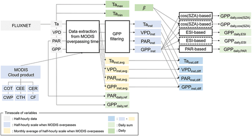
Figure 2. Histograms of the local overpass time for the terra-MODIS and aqua-MODIS. Histogram colors denote the cloudiness of the sky (i.e. clear, cloudy, and ambiguous) at its local overpass time. The cloudiness of the sky was distinguished based on the MODIS cloud mask product (i.e. MOD06 and MYD06).

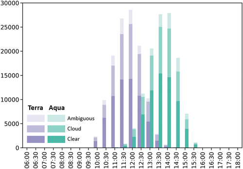
Figure 3. Site-level seasonal correlations between GPP_inst,diff with three environmental variables (PAR_inst,diff—yellow, Ta_inst,diff—red, VPD_inst,diff—blue). The correlation was calculated when the number of samples is larger than 10.

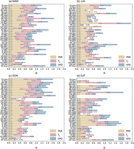
Figure 4. Site-level seasonal correlations between GPP_inst,diff with three environmental variables (PAR_inst,diff—yellow, Ta_inst,diff—red, VPD_inst,diff—blue) under clear and cloudy conditions. The correlation was calculated when the number of samples is larger than 10.

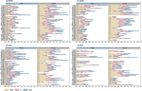
Figure 5. The station-based comparison of slope (refer to Section 3.2) between GPP_daily,ref and the upscaled GPP (i.e. blue: GPP_{daily,cos(SZA)}, purple: GPP_daily,ESI, yellow: GPP_daily,PAR) are presented according to vegetation types: (a) Deciduous broadleaf forests (DBF), (b) Evergreen broadleaf forests (EBF), (c) Evergreen needleleaf forests (ENF), (d) Mixed forests (MF), (e) Grasslands (GRA), and (f) Croplands (CRO). The comparison performed when the number of samples are larger than 10. The x-axis represents the local overpassing time of MODIS divided into one-hour intervals. The y-axis denotes the slope. The red dotted line shows where the slope is 1.

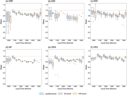
Figure 6. The station-based comparison of R² (referred to section 3.2) between GPP_daily,ref and the upscaled GPP (i.e. blue: GPP_{daily,cos(SZA)}, purple: GPP_daily,ESI, yellow: GPP_daily,PAR) are presented according to vegetation types: (a) deciduous broadleaf forests (DBF), (b) evergreen broadleaf forests (EBF), (c) evergreen needleleaf forests (ENF), (d) mixed forests (MF), (e) grasslands (GRA), and (f) croplands (CRO). The comparison performed when the number of samples are larger than 10. The x-axis represents the local overpassing time of MODIS divided into one-hour intervals. The y-axis denotes the R². The red dotted line shows where the R² is 1.

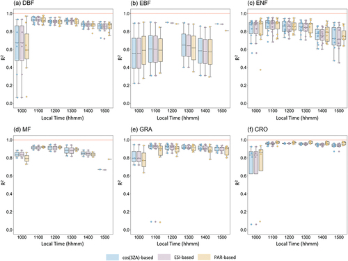
Figure 7. The comparison between the clearness index and the difference between GPP_daily,ref and the three temporal upscaling approaches: (a) cos(SZA)-based, (b) ESI-based, (c) PAR-based. The red represents high point density while the blue indicates low point density.

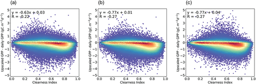
Figure 8. The relationships between GPP_inst,diff and PAR_inst,diff under (a) clear and (b) cloudy sky conditions. Colors indicate the diffuse ratio calculated from the eddy flux data.

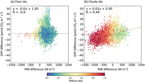
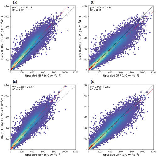
Figure 9. Density plots between the upscaled daily GPP and reference data: (a) GPP_{cos (SZA),daily}, (b) corrected GPP_{cos (SZA),daily}, (c) GPP_ESI,daily, and (d) corrected GPP_ESI,daily.

Wohlfahrt, G., A. Hammerle, A. Haslwanter, M. Bahn, U. Tappeiner, and A. Cernusca. 2008. “Seasonal and Inter-Annual Variability of the Net Ecosystem CO 2 Exchange of a Temperate Mountain Grassland: Effects of Weather and Management.” Journal of Geophysical Research: Atmospheres 113 (D8): D08110. https://doi.org/10.1029/2007JD009286.

 PubMed Web of Science ®Google Scholar

Ammann, C., C. Spirig, J. Leifeld, and A. Neftel. 2009. “Assessment of the Nitrogen and Carbon Budget of Two Managed Temperate Grassland Fields.” Agriculture, Ecosystems & Environment 133 (3–4): 150–162. https://doi.org/10.1016/j.agee.2009.05.006.

 Web of Science ®Google Scholar

Dietiker, D., N. Buchmann, and W. Eugster. 2010. “Testing the Ability of the DNDC Model to Predict CO2 and Water Vapour Fluxes of a Swiss Cropland Site.” Agriculture, Ecosystems & Environment 139 (3): 396–401. https://doi.org/10.1016/j.agee.2010.09.002.

 Web of Science ®Google Scholar

Acosta, M., M. Pavelka, L. Montagnani, W. Kutsch, A. Lindroth, R. Juszczak, D. Janouš 2013. “Soil Surface CO2 Efflux Measurements in Norway Spruce Forests: Comparison Between Four Different Sites Across Europe - from Boreal to Alpine Forest.” Geoderma 192:295–19. https://doi.org/10.1016/j.geoderma.2012.08.027.

 Web of Science ®Google Scholar

Anthoni, P.M., A. Knohl, C. Rebmann, A. Freibauer, M. Mund, W. Mund, O. Mund, E.-D. Schulze 2004. “Forest and Agricultural Land-Use-Dependent CO 2 Exchange in Thuringia, Germany.” Global Change Biology 10 (12): 2005–2019. https://doi.org/10.1111/j.1365-2486.2004.00863.x.

 Web of Science ®Google Scholar

Knohl, A., E. D. Schulze, O. Kolle, and N. Buchmann. 2003. “Large Carbon Uptake by an Unmanaged 250-Year-Old Deciduous Forest in Central Germany.” Agricultural and Forest Meteorology 118 (3–4): 151–167. https://doi.org/10.1016/S0168-1923(03)00115-1.

 Web of Science ®Google Scholar

Grünwald, T., Bernhofer, C. 2007. “A Decade of Carbon, Water and Energy Flux Measurements of an Old Spruce Forest at the Anchor Station Tharandt.”in Tellus, Series B: Chemical and Physical Meteorology 59 (3): 387–396. https://doi.org/10.1111/j.1600-0889.2007.00259.x.

 Web of Science ®Google Scholar

Pilegaard, K., A. Ibrom, M. S. Courtney, P. Hummelshøj, and N. O. Jensen. 2011. “Increasing Net CO2 Uptake by a Danish Beech Forest During the Period from 1996 to 2009.” Agricultural and Forest Meteorology 151 (7): 934–946. https://doi.org/10.1016/j.agrformet.2011.02.013.

 Web of Science ®Google Scholar

Suni, T., Rinne, J., Reissell, A., Altimir, N., Keronen, P., Rannik, Ü., Dal Maso, M., Kulmala, M., Vesala, T. 2003. “Long-Term Measurements of Surface Fluxes Above a Scots Pine Forest in Hyytiälä, Southern Finland, 1996-2001.” Boreal Environment Research 8 (4): 287–301. https://www.borenv.net/BER/archive/ber84.htm.

 Web of Science ®Google Scholar

Aurela, M., L. Annalea, J.-P. Tuovinen, J. Hatakka, T. Penttilä, T. Laurila 2015. “Carbon Dioxide and Energy Flux Measurements in Four Northern-Boreal Ecosystems at Pallas.” Boreal Environment Research 20 (4): 455–473. https://www.borenv.net/BER/archive/ber204.htm.

 Web of Science ®Google Scholar

Berbigier, P., J. M. Bonnefond, and P. Mellmann. 2001. “CO2 and Water Vapour Fluxes for 2 Years Above Euroflux Forest Site.” Agricultural and Forest Meteorology 108 (3): 183–197. https://doi.org/10.1016/S0168-1923(01)00240-4.

 Web of Science ®Google Scholar

Rambal, S., Joffre, R., Ourcival, J.M., Cavender-Bares, J., Rocheteau, A. 2004. “The Growth Respiration Component in Eddy CO 2 Flux from a Quercus Ilex Mediterranean Forest.” Global Change Biology 10 (9): 1460–1469. https://doi.org/10.1111/j.1365-2486.2004.00819.x.

 Web of Science ®Google Scholar

Bonal, D., Bosc, A., Ponton, S., Goret, J.-Y., Burban, B., Gross, P., Bonnefond, J.-M., Elbers, J., Longdoz, B., Epron, D., Guehl, J.-M., Granier, A. 2008. “Impact of Severe Dry Season on Net Ecosystem Exchange in the Neotropical Rainforest of French Guiana.” Global Change Biology 14 (8): 1917–1933. https://doi.org/10.1111/j.1365-2486.2008.01610.x.

 Web of Science ®Google Scholar

Vitale, L., P. Di Tommasi, G. D’Urso, and V. Magliulo. 2016. “The Response of Ecosystem Carbon Fluxes to LAI and Environmental Drivers in a Maize Crop Grown in Two Contrasting Seasons.” International Journal of Biometeorology 60 (3): 411–420. https://doi.org/10.1007/s00484-015-1038-2.

 PubMed Web of Science ®Google Scholar

VALENTINI, R., ANGELIS, P., MATTEUCCI, G., MONACO, R., DORE, S., MUCNOZZA, G.E.S. 1996. “Seasonal Net Carbon Dioxide Exchange of a Beech Forest with the Atmosphere.” Global Change Biology 2 (3): 199–207. https://doi.org/10.1111/j.1365-2486.1996.tb00072.x.

 Web of Science ®Google Scholar

Marcolla, B., A. Cescatti, G. Manca, R. Zorer, M. Cavagna, A. Fiora, D. Gianelle, M. Rodeghiero, M. Sottocornola, and R. Zampedri. 2011. “Climatic Controls and Ecosystem Responses Drive the Inter-Annual Variability of the Net Ecosystem Exchange of an Alpine Meadow.” Agricultural and Forest Meteorology 151 (9): 1233–1243. https://doi.org/10.1016/j.agrformet.2011.04.015.

 Web of Science ®Google Scholar

Migliavacca, M., Meroni, M., Busetto, L., Colombo, R., Zenone, T., Matteucci, G., Manca, G., Seufert, G. 2009. “Modeling Gross Primary Production of Agro-Forestry Ecosystems by Assimilation of Satellite-Derived Information in a Process-Based Model.” Sensors 9 (2): 922–942. https://doi.org/10.3390/s90200922.

 PubMed Web of Science ®Google Scholar

Montagnani, L., G. Manca, E. Canepa, E. Georgieva, M. Acosta, C. Feigenwinter, D. Janous, et al. 2009. “A New Mass Conservation Approach to the Study of CO2 Advection in an Alpine Forest.” Journal of Geophysical Research: Atmospheres 114 (D7): 7306. https://doi.org/10.1029/2008JD010650.

 Google Scholar

TEDESCHI, V., REY, A., MANCA, G., VALENTINI, R., JARVIS, P.G., BORGHETTI, M. 2006. “Soil Respiration in a Mediterranean Oak Forest at Different Developmental Stages After Coppicing.” Global Change Biology 12 (1): 110–121. https://doi.org/10.1111/j.1365-2486.2005.01081.x.

 Web of Science ®Google Scholar

Chiesi, M., F. Maselli, M. Bindi, L. Fibbi, P. Cherubini, E. Arlotta, G. Tirone, G. Matteucci, and G. Seufert. 2005. “Modelling Carbon Budget of Mediterranean Forests Using Ground and Remote Sensing Measurements.” Agricultural and Forest Meteorology 135 (1–4): 22–34. https://doi.org/10.1016/j.agrformet.2005.09.011.

 Web of Science ®Google Scholar

Moors, E.J. 2012. Water Use of Forests in the Netherlands. PhD diss., Vrije Universiteit Amsterdam.

 Google Scholar

Marchesini, L.B., Papale, D., Reichstein, M., Vuichard, N., Tchebakova, N., Valentini, R. 2007. “Carbon Balance Assessment of a Natural Steppe of Southern Siberia by Multiple Constraint Approach.” Biogeosciences 4 (4): 581–595. https://doi.org/10.5194/bg-4-581-2007.

 Web of Science ®Google Scholar

Thomas, C. K., B. E. Law, J. Irvine, J. G. Martin, J. C. Pettijohn, and K. J. Davis. 2009. “Seasonal Hydrology Explains Interannual and Seasonal Variation in Carbon and Water Exchange in a Semiarid Mature Ponderosa Pine Forest in Central Oregon.” Journal of Geophysical Research: Atmospheres 114 (G4): G04006. https://doi.org/10.1029/2009JG001010.

 Google Scholar

Dragoni, D., H. P. Schmid, C. S. B. Grimmond, and H. W. Loescher. 2007. “Uncertainty of Annual Net Ecosystem Productivity Estimated Using Eddy Covariance Flux Measurements.” Journal of Geophysical Research: Atmospheres 112 (D17): D17102. https://doi.org/10.1029/2006JD008149.

 Web of Science ®Google Scholar

Suyker, A. E., S. B. Verma, G. G. Burba, and T. J. Arkebauer. 2005. “Gross Primary Production and Ecosystem Respiration of Irrigated Maize and Irrigated Soybean During a Growing Season.” Agricultural and Forest Meteorology 131 (3–4): 180–190. https://doi.org/10.1016/j.agrformet.2005.05.007.

 Web of Science ®Google Scholar

Desai, A. R., A. Noormets, P. V. Bolstad, J. Chen, B. D. Cook, K. J. Davis, E. S. Euskirchen, et al. 2008. “Influence of Vegetation and Seasonal Forcing on Carbon Dioxide Fluxes Across the Upper Midwest, USA: Implications for Regional Scaling.” Agricultural and Forest Meteorology 148 (2): 288–308. https://doi.org/10.1016/j.agrformet.2007.08.001.

 Web of Science ®Google Scholar

Curtis, P. S., P. J. Hanson, P. Bolstad, C. Barford, J. C. Randolph, H. P. Schmid, and K. B. Wilson. 2002. “Biometric and Eddy-Covariance Based Estimates of Annual Carbon Storage in Five Eastern North American Deciduous Forests.” Agricultural and Forest Meteorology 113 (1–4): 3–19. https://doi.org/10.1016/S0168-1923(02)00099-0.

 Web of Science ®Google Scholar

Ryu, Y., D. D. Baldocchi, S. Ma, and T. Hehn. 2008. “Interannual Variability of Evapotranspiration and Energy Exchange Over an Annual Grassland in California.” Journal of Geophysical Research: Atmospheres 113 (D9): D09104. https://doi.org/10.1029/2007JD009263.

 Web of Science ®Google Scholar

Cook, B. D., K. J. Davis, W. Wang, A. Desai, B. W. Berger, R. M. Teclaw, J. G. Martin, et al. 2004. “Carbon Exchange and Venting Anomalies in an Upland Deciduous Forest in Northern Wisconsin, USA.” Agricultural and Forest Meteorology 126 (3–4): 271–295. https://doi.org/10.1016/j.agrformet.2004.06.008.

 Web of Science ®Google Scholar

Data availability statement

The FLUXNET2015 dataset is available at https://fluxnet.org/data/fluxnet2015-dataset/. The MODIS cloud products (i.e. MOD06_L2 and MYD06_L2) used in this study can be accessed through the NASA LAADS DAAC (https://ladsweb.modaps.eosdis.nasa.gov/search/).