Improving GOCI ocean color data under high solar-zenith angle over open oceans using neural networks

Figures & data

Figure 1. Areas of the studies and examples of the effect of high solar-zenith angle on nL_w(443) for (a) climatology Chl-a image, showing the GOCI field of view: bluish color indicates clear open oceans (climatology Chl-a ≤ 0.3 mg/m³), (b) nL_w(443) image in Box A on February 15, 2020, and (c) the corresponding solar-zenith angle θ₀ image on the same day.

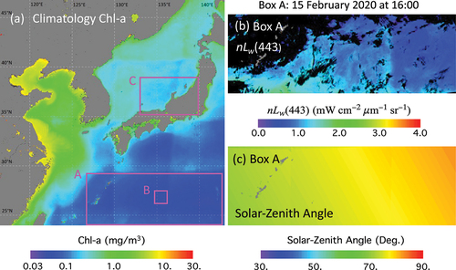
Table 1. Number of training data extracted (number) from years 2011, 2013, 2015, 2017, and 2019 for the NN models for each month and hour combination (month, hour, and NN model name).

Month	Hour	NN model name	Number
January	14:00	Jan1400	4.44×10^5
	15:00	Jan1500	7.33×10^5
	16:00	—	Not enough data
February	14:00	—	Not enough data
	15:00	Feb1500	5.28×10^5
	16:00	Feb1600	5.40×10^5
October	14:00	—	Not enough data
	15:00	Oct1500	7.32×10^5
	16:00	Oct1600	5.12×10^5
November	14:00	Nov1400	5.27×10^5
	15:00	Nov1500	6.88×10^5
	16:00	—	Not enough data
December	14:00	Dec1400	4.64×10^5
	15:00	Dec1500	4.84×10^5
	16:00	—	Not enough data

Figure 2. Diagram of the three-layer fully connected feedforward neural network.

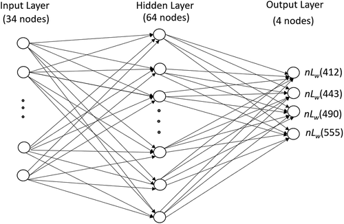
Table 2. List of 34 input variables for the neural network.

Number	Symbol	Description
1	θ	Sensor-zenith angle of the pixel
2–5	θ0	Solar-zenith angles at the correction hour and three previous hours
6–9	Δϕ	Relative-azimuth angles at the correction hour and three previous hours
10–13	W	Wind speeds at the correction hour and three previous hours
14–17	LGN	Glint coefficients at the correction hour and three previous hours
18	hour	hour of measurement for the correction (9–16)
19	day	day of year (1–365)
20	month	month of year (1–12)
21	latitude	latitude of the pixel
22	longitude	longitude of the pixel
23–25	nLw(412)	nLw(412) at the correction hour, two and three hours earlier
26–28	nLw(443)	nLw(443) at the correction hour, two and three hours earlier
29–31	nLw(490)	nLw(490) at the correction hour, two and three hours earlier
32–34	nLw(555)	nLw(555) at the correction hour, two and three hours earlier

Figure 3. The GOCI-measured original nL_w(412), nL_w(443), nL_w(490), and nL_w(555) images of Box B (noted in Figure 1a) at 12:00 to 16:00 on February 3, 2020 (first five columns). The last two columns are the NN-corrected $\mathit{n}{L}_w^{\left(C\right)}$(λ) images at 15:00 and 16:00.

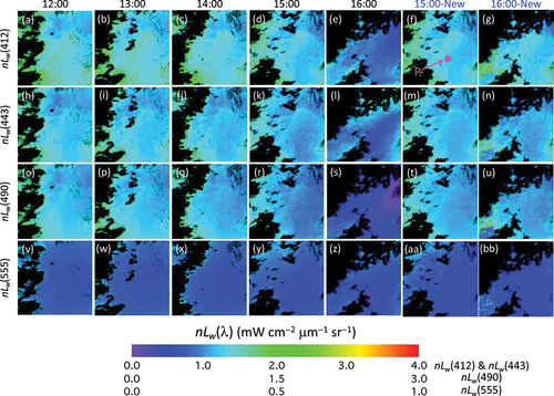
Figure 4. Hourly time series (09:00–16:00) of original nL_w(412), nL_w(443), nL_w(490), and nL_w(555) (solid lines), and the corresponding NN-corrected $\mathit{n}{L}_w^{\left(C\right)}$(λ) (dashed lines) at the location P in Figure 3f on February 3, 2020.

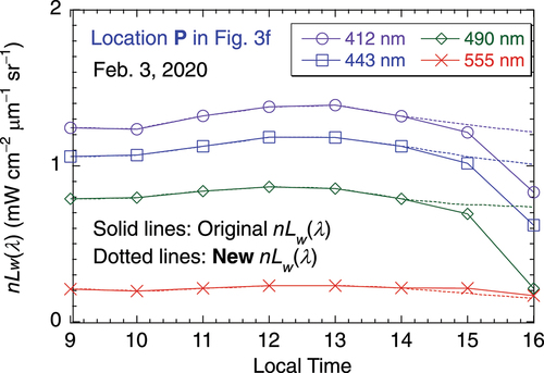
Figure 5. Scatter/density plots of GOCI-derived original nL_w(λ, θ₀>65°, 16) (top row), original nL_w(λ, θ₀≤65°, 16) (middle row), and new $\mathit{n}{L}_w^{\left(C\right)}$(λ, θ₀>65°, 16) (bottom row) versus original nL_w(λ, θ₀≤65°, 15) at spectral bands of 412, 443, 490, and 555 nm in the month of February 2020. The statistics show that nL_w(λ, θ₀>65°, 16) are underestimated by 15–30% for blue bands, and overestimated by 17% for green band. After correction, the ratio r^(C)(λ, ≤65°, >65°, 15, 16) is close to the reference r(λ, ≤65°, ≤65°, 15, 16).

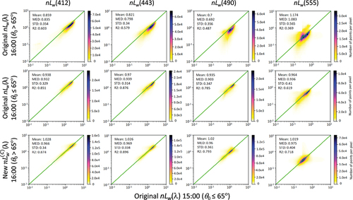
Table 3. Evaluation results of r(λ, θ_0, θ₀′, t, t′) and r^(C)(λ, θ₀, θ₀′, t, t′) (mean, median, and STD) for the month of February 2020.

Ratio r(λ, θ0, θ0′, t, t′) or r^(C)(λ, θ0, θ0′, t, t′)	412 nm			443 nm			490 nm			555 nm
	Mean	Median	STD	Mean	Median	STD	Mean	Median	STD	Mean	Median	STD
r(λ, ≤65°, >65°, 15, 16)	0.859	0.835	0.354	0.821	0.798	0.340	0.700	0.692	0.356	1.174	1.083	0.565
r(λ, ≤65°, ≤65°, 15, 16)	0.938	0.932	0.329	0.970	0.939	0.314	0.935	0.903	0.347	0.964	0.936	0.410
r^(C)(λ, ≤65°, >65°, 15, 16)	1.028	0.966	0.340	1.026	0.969	0.334	1.020	0.960	0.361	1.019	0.975	0.404
r(λ, ≤65°, >65°, 14, 15)	0.942	0.912	0.344	0.922	0.897	0.336	0.821	0.817	0.384	1.063	0.948	0.554
r(λ, ≤65°, ≤65°, 14, 15)	0.984	0.973	0.224	0.992	0.975	0.229	0.969	0.948	0.273	1.041	1.057	0.333
r^(C)(λ, ≤65°, >65°, 14, 15)	1.024	0.969	0.336	1.021	0.967	0.328	1.016	0.971	0.354	1.020	0.996	0.451

Figure 6. Scatter/density plots of GOCI-derived original nL_w(λ) (top row), new $\mathit{n}{L}_w^{\left(C\right)}$(λ) (middle row), and ratio of new $\mathit{n}{L}_w^{\left(C\right)}$(λ)/original nL_w(λ) (bottom row) on February 3, 2020, as a function of solar-zenith angle (θ₀).

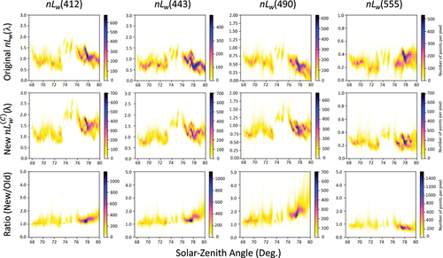
Figure 7. GOCI-measured original nL_w(412), nL_w(443), nL_w(490), and nL_w(555) images of Box C noted in Figure 1a from 12:00–15:00 on November 5, 2014 (first four columns). The last two columns are for the NN-corrected $\mathit{n}{L}_w^{\left(C\right)}$(λ) images at 14:00 and 15:00, respectively.

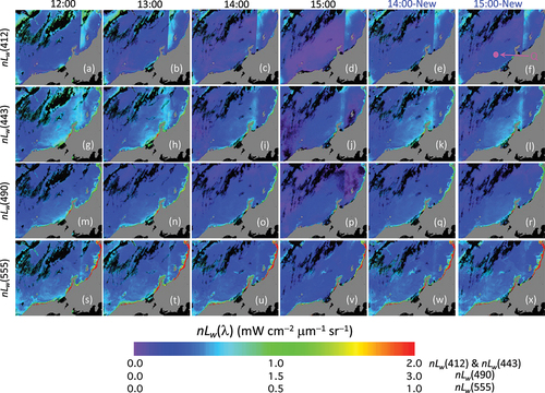
Figure 8. Hourly time series (09:00–15:00) of original nL_w(412), nL_w(443), nL_w(490), and nL_w(555) (solid lines), and the corresponding NN-corrected $\mathit{n}{L}_w^{\left(C\right)}$(λ) (dashed lines) at the location Q noted in Figure 7f on November 5, 2014.

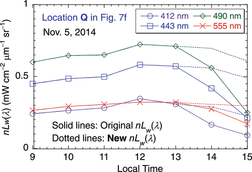
Figure 9. Scatter/density plots of GOCI-derived original nL_w(λ, θ₀>65°, 15) (top row), original nL_w(λ, θ₀ ≤65°, 15) (middle row), and new $\mathit{n}{L}_w^{\left(C\right)}$(λ, θ₀>65°, 15) (bottom row) versus original nL_w(λ, θ₀≤65°, 14) from the region in Box C (noted in Figure 1a) at spectral bands of 412, 443, 490, and 555 nm for the month of November 2014. The statistics show that nL_w(λ, θ₀>65°, 15) are underestimated by 13–21% for blue bands, and overestimated by 16% for green band. After correction, the ratio r^(C)(λ, ≤65°, >65°, 14, 15) is close to the reference r(λ, ≤65°, ≤65°, 14, 15).

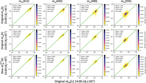
Table 4. Evaluation results r(λ, θ_0, θ₀′, t, t′) and r^(C)(λ, θ₀, θ₀′, t, t′) (mean, median, and STD) for the month of November 2014.

Ratio r(λ, θ0, θ0′, t, t′) or r^(C)(λ, θ0, θ0′, t, t′)	412 nm			443 nm			490 nm			555 nm
	Mean	Median	STD	Mean	Median	STD	Mean	Median	STD	Mean	Median	STD
r (λ, ≤65°, >65°, 14, 15)	0.869	0.859	0.324	0.867	0.865	0.338	0.787	0.793	0.384	1.162	1.135	0.551
r (λ, ≤65°, ≤65°, 14, 15)	0.985	0.973	0.265	0.993	0.974	0.273	0.942	0.923	0.321	1.056	1.042	0.392
r^(C)(λ, ≤65°, >65°, 14, 15)	0.986	0.945	0.284	0.997	0.950	0.298	1.005	0.950	0.332	1.011	0.964	0.398
r (λ, ≤65°, >65°, 13, 14)	0.936	0.922	0.336	0.936	0.925	0.342	0.827	0.829	0.378	1.170	1.037	0.515
r (λ, ≤65°, ≤65°, 13, 14)	1.017	1.010	0.310	1.030	1.014	0.290	1.018	0.993	0.317	1.047	1.014	0.364
r^(C)(λ, ≤65°, >65°, 13, 14)	1.008	0.959	0.293	1.024	0.967	0.307	1.024	0.961	0.343	1.018	0.974	0.434

Table 5. Evaluation results r(λ, θ_0, θ₀′, t, t′) and r^(C)(λ, θ₀, θ₀′, t, t′) (mean, median, and STD) for all five months (January, February, October, November, and December) and in all five even years (2012, 2014, 2016, 2018, and 2020).

Ratio r (λ, θ0, θ0′, t, t′) or r^(C)(λ, θ0, θ0′, t, t′)	412 nm			443 nm			490 nm			555 nm
	Mean	Median	STD	Mean	Median	STD	Mean	Median	STD	Mean	Median	STD
r (λ, ≤65°, >65°, 15, 16)	0.899	0.871	0.399	0.890	0.875	0.394	0.817	0.806	0.412	1.145	1.094	0.604
r (λ, ≤65°, ≤65°, 15, 16)	0.988	0.974	0.314	0.977	0.976	0.312	0.932	0.917	0.345	1.047	1.030	0.406
r^(C)(λ, ≤65°, >65°, 15, 16)	1.027	0.986	0.351	1.025	0.984	0.347	1.045	1.002	0.376	0.968	0.952	0.441
r (λ, ≤65°, >65°, 14, 15)	0.947	0.924	0.388	0.937	0.928	0.378	0.926	0.909	0.404	1.089	1.045	0.569
r (λ, ≤65°, ≤65°, 14, 15)	0.981	0.966	0.324	0.984	0.965	0.321	0.964	0.945	0.341	1.028	1.012	0.436
r^(C)(λ, ≤65°, >65°, 14, 15)	1.015	0.999	0.342	1.005	0.993	0.345	1.013	0.996	0.360	1.009	1.001	0.453
r (λ, ≤65°, >65°, 13, 14)	0.953	0.964	0.392	0.963	0.947	0.391	0.950	0.937	0.416	1.063	1.031	0.493
r (λ, ≤65°, ≤65°, 13, 14)	0.984	0.974	0.333	0.989	0.980	0.316	0.978	0.968	0.346	1.030	1.020	0.422
r^(C)(λ, ≤65°, >65°, 13, 14)	1.018	0.997	0.358	1.001	1.011	0.356	1.004	0.979	0.360	1.005	0.995	0.450

Figure 10. Comparison of GOCI-derived (a) original Chl-a and (b) new Chl-a in the region of Box A in Figure 1a on February 15, 2020.

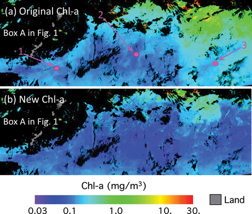
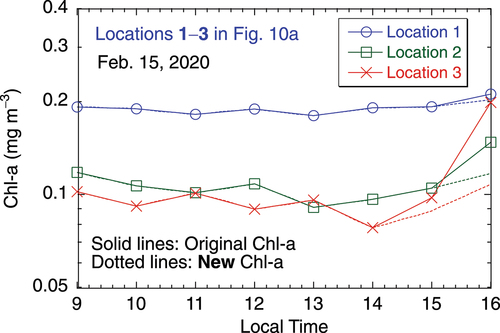
Figure 11. Comparison of hourly time series (09:00–16:00) for the GOCI-derived original Chl-a (solid lines) and new Chl-a (dashed lines) at the locations 1, 2, and 3 defined in Figure 10a on February 15, 2020.

Data availability statement

The data that support the findings of this study are available from the corresponding author upon reasonable request.