High-dimensional detection of Landscape Dynamics: a Landsat time series-based algorithm for forest disturbance mapping and beyond

Figures & data

Figure 1. Geographic location of the study area and validation plots with information from the Dominant Leaf Type 2018 forest cover layer (European Environmental Agency 2020) and Landsat Path/Row coverage (World Reference System 2). The base layer corresponds to the hill shade derived from the 25 m EU-DEM digital surface model.

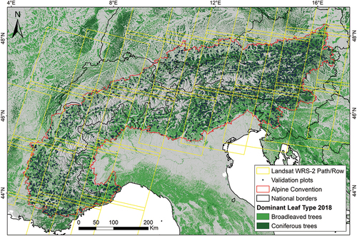
Table 1. List of the spectral indices used in this study.

Index	Formulation	Direction of change caused by a disturbance	Reference
Normalized Difference Vegetation Index (NDVI)	(NIR – Red)/(NIR + Red)	decrease	(Rouse et al. 1973)
Normalized Difference Moisture Index (NDMI)	(NIR – SWIR1)/(NIR + SWIR1)	decrease	(Wilson and Sader 2002)
Normalized Burn Ratio (NBR)	(NIR – SWIR2)/(NIR + SWIR2)	decrease	(García and Caselles 1991)
Moisture Stress Index (MSI)	NIR/SWIR1	increase	(Hunt and Rock 1989)
Tasseled Cap Brightness (TCB)	0.3037*Blue+0.2793*Green+0.4743*Red+0.5585*NIR+0.5082*SWIR1+0.1863*SWIR2	increase	(Crist 1985)
Tasseled Cap Greenness (TCG)	−0.2848*Blue−0.2435*Green−0.4743*Red+0.7243*NIR+0.0840*SWIR1−0.1800*SWIR2	decrease	(Crist 1985)
Tasseled Cap Wetness (TCW)	0.1509*Blue+0.1973*Green+0.3279*Red+0.34065*NIR−0.7112*SWIR1−0.4572*SWIR2	decrease	(Crist 1985)
Tasseled Cap Angle (TCA)	arctan(TCB/TCG)	decrease	(Powell et al. 2010)

Figure 2. Flowchart of the main operations performed by HILANDYN. Input data consist of four-dimensional raster cubes where bands and time form the third and fourth dimensions, respectively. A three-dimensional spatial kernel is employed on a pixel basis to build $\mathit{n}$-dimensional time series with a matrix form of the dimension $\mathit{n}\times \mathit{T}$. The core operations performed by HILANDYN on $\mathit{n}$-dimensional time series are described in the orange box.

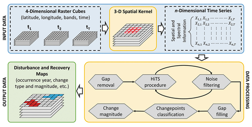
Figure 3. Examples of the spatial arrangement of disturbed pixels (orange) within the spatial kernel used by HILANDYN where the focal pixel is surrounded by non-disturbed pixels (grey).

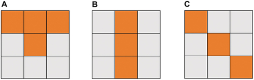
Figure 4. Example of time series of three focal pixels containing sparse noise (a), dense noise (b) or spectral changes caused by a wildfire (c). HILANDYN ignored sparse noise (a) while detected the dense ones in 1986 and 2002 (b). The wildfire occurred in 1991 (c) caused a changepoint characterised by a spike similar to impulsive noise though some bands, i.e. SWIR1, SWIR2 and TCW, did not exhibit a rapid spectral recovery.

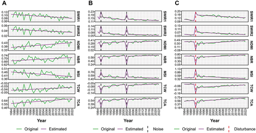
Figure 5. Diagram of the operations performed by the noise filter during the screening stage for each interval. The number of observations per year and the parameter $\mathit{nob}\_{init}_{min}$ are required for evaluating condition $C_1$. Original and estimated spectral values are required for evaluating conditions $C_2$ and $C_3$. Time points at the beginning of the time series are first processed through condition $C_1$. Conditions $C_2$ and $C_3$ are checked on time points that exhibit the maximal spectral deviation from a reference value. Blue boxes indicate input data, black boxes indicate processing and green boxes indicate outputs.

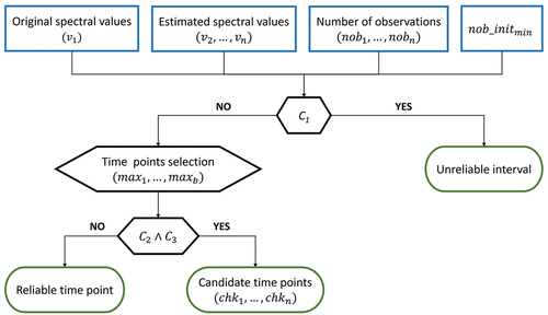
Table 2. Information on the validation dataset based on the validation strata. We discriminated between stand-replacing and non-stand-replacing events using a threshold of 50% of the relative TCW change magnitude.

Validation stratum	Total plots	Disturbed plots	Stand-replacing events	Non-stand-replacing events
Inner	1500	1439	1268	632
Outer	1500	706	408	494
Inner and outer	3000	2145	1676	1126

Table 3. List of the main parameters required by HILANDYN and values tested for the sensitivity analysis.

Parameters	Tested alternatives or values
Input bands	All the unique combinations with length in the interval [1, 14], obtained using six original Landsat bands (Blue, Green, Red, NIR, SWIR1, SWIR2) and spectral indices listed in Table 1.
Constant $\mathit{C}$	Values in the interval [0.6, 1.2] increased by 0.2.
$\mathit{noise}\_\mathit{ite}{r}_{\mathit{max}}$	Values in the interval [0, 4] increased by 1.
$\mathit{nob}\_\mathit{ini}{t}_{\mathit{min}}$	Values in the interval [2, 10] increased by 1.

Figure 6. Maximum values of user’s accuracy (UA), producer’s accuracy (PA) and F₁ score based on the validation dataset and computed from all the unique combinations of bands with lengths from one to 14. The value of the constant $\mathit{C}$ ranged from 0.6 to 1.2. The noise filter was deactivated.

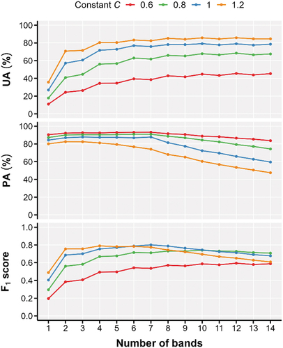
Figure 7. Distribution of values of user’s accuracy (UA), producer’s accuracy (PA) and F₁ score based on the validation dataset and computed from all the unique combinations of bands with lengths from one to 14. The value of the constant factor $\mathit{C}$ was equal to one. The noise filter was deactivated.

Figure 8. Frequency count relative to the number of times each band was in the best-performing combination in terms of PA, using from one to 14 bands in the high-dimensional time series. Results obtained with values of the constant factor $\mathit{C}$ ranging from 0.6 to 1.2 were pooled together. The noise filter was deactivated.

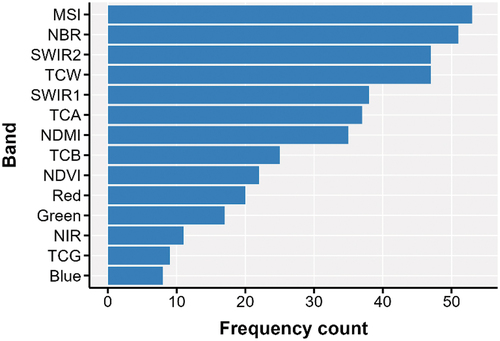
Table 4. User’s accuracy (UA), producer’s accuracy (PA), and F₁ score achieved by HILANDYN with the noise filter activated or not. Accuracy metrics were computed using either both strata of the validation dataset or a single one. High-dimensional Landsat time series included data from seven bands (SWIR1, SWIR2, NDMI, NBR, MSI, TCW, and TCA) within a three-by-three spatial kernel. We parametrized the algorithm using $\mathit{C}$ = 1, $\mathit{noise}\_\mathit{ite}{r}_{\mathit{max}}$ = 4, and $\mathit{nob}\_\mathit{ini}{t}_{\mathit{min}}$ = 5.

Validation stratum	Noise unfiltered			Noise filtered
	UA (%)	PA (%)	F1 score	UA (%)	PA (%)	F1 score
Inner	80.9	92	0.861	87.5	88.7	0.881
Outer	60.5	78.9	0.685	73.5	72.4	0.730
Inner and outer	73.7	87.8	0.801	83.1	83.5	0.833

Figure 9. Distribution of the relative TCW change magnitude of commission (100 – UA) errors and omission (100 – PA) errors for HILANDYN and BEAST. High-dimensional Landsat time series included data of seven bands (SWIR1, SWIR2, NDMI, NBR, MSI, TCW and TCA) within a three-by-three spatial kernel. We parametrised each algorithm using the settings that provided the best results in terms of F₁ score. We constrained the relative TCW change magnitude between −50% and 250% by assigning these values to those outside that range.

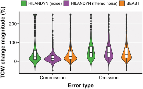
Table 5. User’s accuracy (UA), producer’s accuracy (PA), and F₁ score achieved by BEAST with the validation dataset as a function of the maximum number of trend changepoints (trendMaxKnotNum) and the data in the time series. Input time series included either data of one band (NBR), or seven bands (SWIR1, SWIR2, NDMI, NBR, MSI, TCW, and TCA) of one or nine pixels, i.e. within a three-by-three spatial kernel. The highest value of each accuracy metric for every input data type is highlighted in bold.

Maximum number of trend changepoints (trendMaxKnotNum)	One band (one pixel)			One band (nine pixels)			Seven bands (one pixel)			Seven bands (nine pixels)
	UA (%)	PA (%)	F1 score	UA (%)	PA (%)	F1 score	UA (%)	PA (%)	F1 score	UA (%)	PA (%)	F1 score
1	65.1	53.0	0.584	70.7	57.4	0.634	69.3	58.8	0.636	73.0	62.5	0.674
2	65.0	52.9	0.584	70.9	57.6	0.635	69.0	58.4	0.633	73.1	62.7	0.675
3	58.9	64.1	0.614	64.3	73.2	0.684	62.7	71.9	0.669	67.2	76.9	0.717
4	50.2	68.4	0.579	54.8	78.6	0.646	53.6	77.5	0.633	55.3	82.5	0.662
5	46.0	70.1	0.555	51.1	80.4	0.625	49.4	79.0	0.608	52.7	84.4	0.648
6	44.0	70.7	0.542	48.9	81.2	0.611	47.6	79.4	0.595	50.7	85.3	0.636
7	43.2	70.9	0.537	47.9	81.6	0.604	46.8	79.4	0.589	49.9	85.5	0.630
8	43.1	71.0	0.536	48.1	82.1	0.607	46.8	80.0	0.590	49.6	85.6	0.628
9	43.0	71.2	0.536	48.0	81.7	0.605	46.7	79.7	0.589	49.5	85.8	0.628
10	42.8	70.8	0.534	47.6	81.7	0.601	46.5	79.7	0.587	49.7	85.7	0.629

Figure 10. Execution time required by HILANDYN and BEAST to process the 39-year high-dimensional time series of the validation dataset. The total number of variables in each time series was equal to the product of the number of bands and nine, i.e. the number of pixels within a three-by-three spatial kernel. The bands selected in each combination were those that gave the best results in terms of PA with HILANDYN when the constant $\mathit{C}$ was equal to one (Table S1). We configured the noise filter of HILANDYN by setting the $\mathit{noise}\_\mathit{ite}{r}_{\mathit{max}}$ to four and $\mathit{nob}\_\mathit{ini}{t}_{\mathit{min}}$ to five. For BEAST, we used the predefined prior parameters except for trendMaxknotnum and trendMinsepdist that we set to eight and one, respectively. Each process ran on a single core of an AMD Ryzen 9 5950X processor.

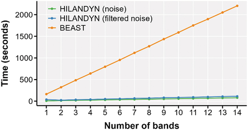
Figure 11. Examples of stand-replacing and non-stand-replacing forest disturbances detected by HILANDYN in the study area between 1985 and 2022. Panels A-F depict the following disturbance events: (a) dieback induced by defoliating insect outbreak (Asian chestnut gall wasp, Dryocosmus kuriphilus) in 2011; (b) dieback caused by a severe drought and heatwave in 2003; (c) wildfires in 1990, 1991, 2003, and 2017; (d) windthrow in 2007; (e) ice storm in 2014; (f) windthrow in 2018. The grey background in the central panel indicates the presence of forest cover either in 1990 or 2018 according to the Corine Land Cover within the European Alps borders (blue line).

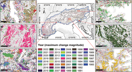
Figure 12. Examples of disturbed forest patches detected by HILANDYN and characterised by different disturbance agents and severities. Please refer to the legend in Figure 11 for the colour corresponding to each year in panels a-e. Clearcuts (a, f; 5°45‘18,102“E; 44°3’9,791“N), debris flows (b, g; 8°1‘54,389“E; 46°46’4,057“N), defoliating insect outbreak (c, h; 7°35‘10,709“E; 45°22’18,178“N), wildfire (d, i; 13°16‘54,707“E; 46°28’25,202“N), windthrow (e, j; 7°21‘17,61“E; 44°39’31,641“N). The grey background indicates the presence of forest cover either in 1990 or 2018 according to the Corine Land Cover.

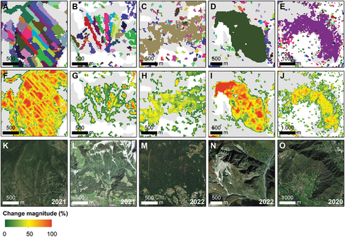
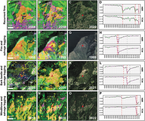
Figure 13. Examples of forest patches, depicted in yellow, that were disturbed multiple times during the analysis period. Each row shows results from HILANDYN, recent high-resolution satellite imagery, and temporal profiles of NBR and TCW. We parametrised the algorithm according to the configuration that achieved the highest F₁ score (Section 3.1). Recurrent wildfires (a-d; 7° 9’1.02“E; 45° 9’35.57“N). Wildfire followed by salvage logging (e-h; 9°39’23.26“E; 46°11’59.51“N). Bark beetle attack followed by salvage logging (i-l; 14°42’0.63“E; 46°16’1.43“N). Windthrow followed by salvage logging (m-p; 11°21’13.93“E; 46°17’41.66“N).

European Environmental Agency. 2020. “Copernicus Land Monitoring Service – Dominant Leaf Type 2018 [WWW Document]. URL https://land.copernicus.eu/pan-european/high-resolution-layers/forests/dominant-leaf-type.( Accessed June 1, 2021).

 Google Scholar

Rouse, J. W., R. H. Hass, J. A. Schell, and D. W. Deering. 1973. “Monitoring Vegetation Systems in the Great Plains with ERTS.” Third Earth Resour Technol Satell Symp 1:309–317. h ttps://d oi.org/citeulike-article-id:12009708.

 Google Scholar

Wilson, E. H., and S. A. Sader. 2002. “Detection of Forest Harvest Type Using Multiple Dates of Landsat TM Imagery.” Remote Sensing of Environment 80 (3): 385–396. https://doi.org/10.1016/S0034-4257(01)00318-2.

 Web of Science ®Google Scholar

García, M. J. L., and V. Caselles. 1991. “Mapping Burns and Natural Reforestation Using Thematic Mapper Data.” Geocarto International 6 (1): 31–37. https://doi.org/10.1080/10106049109354290.

 Google Scholar

Hunt, E. R., Jr, and B. N. Rock. 1989. “Detection of Changes in Leaf Water Content Using Near-And Middle-Infrared Reflectances.” Remote Sensing of Environment 30 (1): 43–54. https://doi.org/10.1016/0034-4257(89)90046-1.

 Web of Science ®Google Scholar

Crist, E. P. 1985. “A TM Tasseled Cap Equivalent Transformation for Reflectance Factor Data.” Remote Sensing of Environment 17 (3): 301–306. https://doi.org/10.1016/0034-4257(85)90102-6.

 Web of Science ®Google Scholar

Powell, S. L., W. B. Cohen, S. P. Healey, R. E. Kennedy, G. G. Moisen, K. B. Pierce, and J. L. Ohmann. 2010. “Quantification of Live Aboveground Forest Biomass Dynamics with Landsat Time-Series and Field Inventory Data: A Comparison of Empirical Modeling Approaches.” Remote Sensing of Environment 114 (5): 1053–1068. https://doi.org/10.1016/j.rse.2009.12.018.

 Web of Science ®Google Scholar

Data availability statement

The code of the algorithm is implemented in the R package “hilandyn” publicly available via the GitHub repository of the first author at https://github.com/donatomorresi/hilandyn.