
Figures & data
Figure 1. Maps of important features of Pennsylvania, USA. (A) Public forests (green) and areas of interest for conservation (purple), (B) LiDAR delivery areas described in , (C) airborne LiDAR survey dates, and (D) Google Eath Engine Dynamic World land cover (Brown et al. Citation2022).
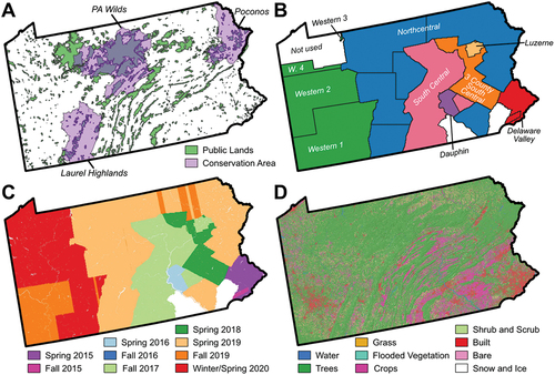
Table 1. Relevant technical and data acquisition specifics of airborne LiDAR used in this work.
Table 2. Descriptions of all LiDAR metrics considered for use in the predictive model.
Figure 2. Airborne LiDAR tiles with point return height normalized to the ground surface depicting the four different timber harvest types and ages that the XGBoost model was trained to identify. (A) Two typical overstory removal plots (2-year old and 11-year old) along with intact mature forest (untreated class) (from −77.578°W, 41.653°N). Notice the ingrowth of the understory in the older overstory removal compared to the more recent plot. (B) Two 7-year old shelterwood harvest plots showing the systematic canopy gaps typical of such harvests (from −77.929°W, 40.968°N). (C) A rare 14-year old shelterwood harvest still displaying some of the same gap structure as shown in (B) (from −77.956°W, 41.291°N).
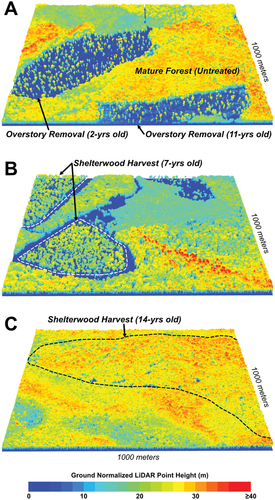
Figure 3. (A) state timber harvest data used for training and testing the XGBoost model (magenta) with a zoomed in example in (B). The speckled white areas in (B) are the decimated samples of the “untreated” forest class and the stars indicate two examples of locations where timber harvest postdated LiDAR data collection and were not used (colorless patches). Private forests shown in (A) were derived from the Dynamic World dataset (Brown et al. Citation2022).
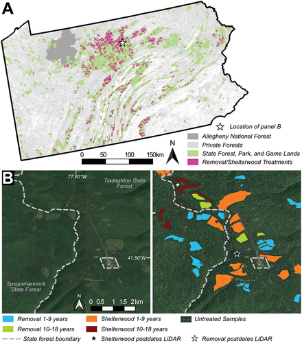
Figure 4. Violin plots showing the dependence of forest structure on forest management type and harvest age. Shown are two metrics of forest structure: (A) the percent of LiDAR returns <2m from the ground (V2), and (B) the height of the 95-th percentile return (p95). Note that the training data contains no shelterwood older than 18 years. Hashes inside the violin plots denote the inter-quartile range and median for each distribution.
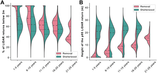
Table 3. XGBoost hyperparameters tuned using a grid search to produce the optimal model.
Table 4. Confusion matrix showing correct classification rates (diagonal elements) and error rates (off diagonal elements).
Figure 5. Receiver operating characteristic (ROC) plots and Area Under the Curve (AUC) for each class modeled. The threshold indicated for each class (circles) balances false and true positive error rates.
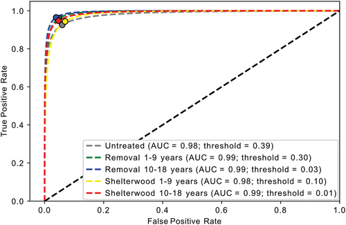
Figure 6. Final classification map for two areas with exemplar forest harvests of both types and ages occurring on both sides of the private-public boundary. Comparison with airborne photography shows that many of the harvests mapped are not apparent in optical data. In other cases, harvested areas show up as areas with less shading (lighter) or more non-photosynthetic vegetation (browner) in aerial photos.
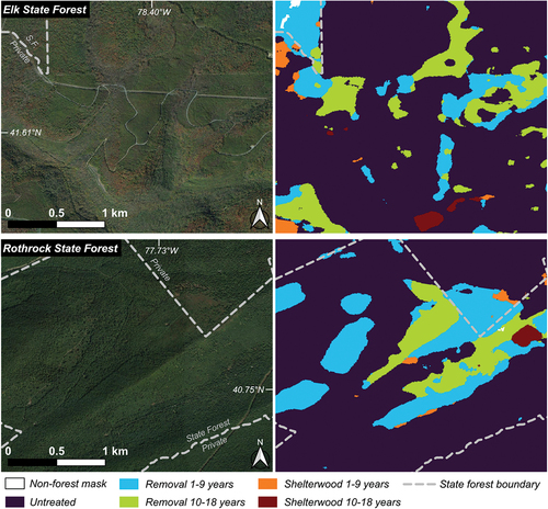
Figure 7. Predicted results for the PA wilds conservation area.
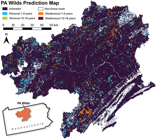
Figure 8. The top 10 most important metrics for each harvest class based on the mean SHAP values (Lundberg et al. Citation2020) from the XGBoost model. See for definitions of each metric.
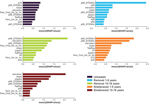
Table 5. Statistics for public and private forest lands for each class in the three key conservation areas across Pennsylvania.
Data availability statement
Due to the considerable size of (1) the data that support the findings of this study and (2) the resulting products, these data are only available from the corresponding author, G. Burch Fisher, upon reasonable request. All code associated with this project and specific package parameters needed for reproducibility can be found in the public GitHub repository for the project (https://github.com/burchfisher/ForestBirds).